One-Hot Encoding: Breaking the Code for Categories

I. Introduction

In the world of machine learning and data science, it’s essential to speak the same language as your computer. Unfortunately, computers don’t understand words and categories in the same way humans do. Computers prefer numbers, and this is where “One-Hot Encoding” comes into play.

Definition of One-Hot Encoding

One-hot encoding is a process of converting categorical data variables so they can be provided to machine learning algorithms to improve predictions. With one-hot, we transform each category value into a new column and assign a 1 or 0 (True/False) value to the column. This has the benefit of not weighting a value improperly but does have the downside of adding more columns to the data set.

For instance, imagine you have a “color” variable which can be “red”, “blue”, or “green”. One-Hot Encoding transforms this into three variables: “is_red”, “is_blue”, and “is_green”, each of which is either 1 or 0.

Understanding Categorical Variables

A categorical variable is a variable that can take on one of a limited number of categories. For example, if we have a data field called “Weather”, it may contain categories such as “sunny”, “cloudy”, “rainy”, and “foggy”. Categorical variables are often words, not numbers, but machine learning algorithms usually require numbers. That’s why we need One-Hot Encoding.

Overview of One-Hot Encoding

One-Hot Encoding is a two-step process:

1. We first convert the categorical variable into an integer-encoded variable, where each category is represented by a unique integer.
2. Next, each of these integers is then converted into a binary form – a series of 0s and 1s.

This binary output ensures that the machine learning algorithm doesn’t mistakenly assume that there’s an ordered relationship between categories when there isn’t one.

Importance of One-Hot Encoding in Data Science

One-Hot Encoding is critical for handling categorical variables in many machine learning algorithms. Without it, your algorithm might assume that two nearby values are more similar than two distant ones, which is often incorrect. For instance, if “red” is 1, “blue” is 2, and “green” is 3, a machine might think that red is more similar to blue than green, which doesn’t make sense.

Now that we’ve introduced One-Hot Encoding, let’s dig deeper into how it compares with other encoding techniques, its core concepts, and its practical application in Python.

II. One-Hot Encoding vs Other Encoding Techniques

Even though One-Hot Encoding is a very popular method to handle categorical data, there are other techniques as well. Let’s discuss three of them: Label Encoding, Ordinal Encoding, and Binary Encoding. We’ll see what makes each one special and how they are different from One-Hot Encoding.

One-Hot Encoding vs Label Encoding

Label Encoding is a way of converting each category value of a variable into a number. So if your variable is “color” and the options are “red”, “blue”, and “green”, Label Encoding might give “red” a 1, “blue” a 2, and “green” a 3. The problem is, the machine might think that “green” is greater than “blue”, and “blue” is greater than “red”, which is not true! Colors don’t have a greater or lesser value, they are just different. So this is where One-Hot Encoding is very helpful. It creates new variables for each category, and doesn’t give one a bigger number than another.

One-Hot Encoding vs Ordinal Encoding

Now, Ordinal Encoding is slightly different from Label Encoding. It still converts categories into numbers, but this time the order does matter. For example, if your variable is “mood” and the options are “happy”, “neutral”, and “sad”, Ordinal Encoding might give “sad” a 1, “neutral” a 2, and “happy” a 3. Here the numbers do have meaning: a higher number means a happier mood. Ordinal Encoding is great for categories that have an order, but it’s not so good for categories like colors that don’t have a logical order. So, again, in such cases, One-Hot Encoding is a better choice.

One-Hot Encoding vs Binary Encoding

Lastly, let’s look at Binary Encoding. In this technique, categories are first converted into numeric labels just like Label Encoding, but then those numeric labels are converted into binary code. So “red”, “blue”, and “green” might become 1, 2, and 3, and then 01, 10, and 11. This can be very efficient when you have many categories, as it doesn’t create as many new variables as One-Hot Encoding does. But on the downside, it might not be as easy for a machine to learn from Binary Encoded data compared to One-Hot Encoded data.

So, as you can see, each encoding technique has its strengths and weaknesses, and the choice between them depends on the specific task and the specific data you have.

III. Deep Dive into One-Hot Encoding

Concept and Basics

In simple terms, One-Hot Encoding is like spreading out your categories into many buckets, where each bucket is either full or empty. If a category is present, we say its bucket is full (marked as 1), and if it’s not, its bucket is empty (marked as 0).

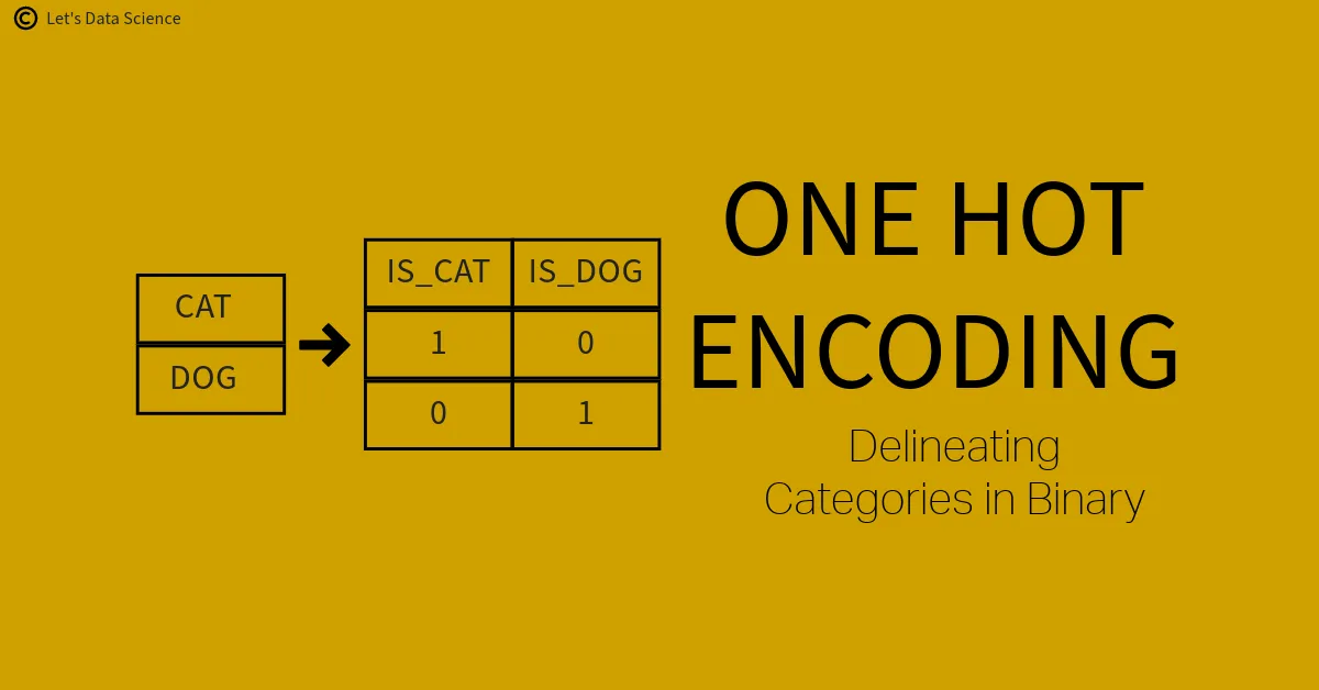
Let’s say we have some animals: “cat”, “dog”, “fish”. In One-Hot Encoding, each of these animals would get its own bucket. So if we have a “cat”, we fill the “cat” bucket (mark it as 1), and leave the “dog” and “fish” buckets empty (mark them as 0). This way, every animal gets represented uniquely, and it’s easy to see which animal we have just by looking at which bucket is full.

One thing to remember here is that in One-Hot Encoding, each category becomes a new column in our data. So if we have 10 categories, we’ll end up with 10 new columns. This can make our data much larger, but it’s worth it because it helps our computer understand the data better.

Mathematical Foundation

Mathematically, One-Hot Encoding involves representing each category as a vector. A vector is just a list of numbers. In our case, the vector has a length equal to the number of categories we have. Each position in the vector represents a category. When a category is present, we put a 1 in its position in the vector, and put 0s in all the other positions.

Let’s go back to our animal example. We can represent “cat”, “dog”, and “fish” as vectors like this:

• Cat: [1, 0, 0]
• Dog: [0, 1, 0]
• Fish: [0, 0, 1]

This is the mathematical foundation of One-Hot Encoding. It’s a way of representing categories as vectors, where each vector is unique and clearly shows which category it represents.

Advantages and Disadvantages

One big advantage of One-Hot Encoding is that it removes any sense of order from the categories. This is great when the order doesn’t matter, like with our animals. The computer won’t think that a “fish” is somehow “greater” than a “dog” just because “fish” comes after “dog” in our list.

Another advantage is that One-Hot Encoding can make it easier for certain machine learning models to learn. Since each category gets represented uniquely, the model can focus on learning from the features of each category individually.

But there are also disadvantages to One-Hot Encoding. As we saw earlier, it can make our data much larger because it adds new columns. If we have a category with many unique values, our data might become too large to handle! This is called the “curse of dimensionality”.

Another downside is that One-Hot Encoding can be harder to interpret. If we have many categories, it might be hard to understand what’s going on with all those 0s and 1s.

The Problem of Dimensionality and Sparse Vectors

A problem that can occur when using One-Hot Encoding is creating data with too many dimensions. This is often referred to as high-dimensional data, which can be hard to visualize and manage.

Also, the vectors produced by One-Hot Encoding can often be very sparse. This means they contain a lot of zeros and only one one. For example, if you have 1000 categories and are encoding category number 500, the resulting vector will have one ‘1’ and 999 ‘0s’.

Sparse data can sometimes be problematic for machine learning algorithms as it might lead to overfitting, where the model learns the training data too well and performs poorly on unseen data.

Despite these challenges, One-Hot Encoding is a powerful tool in a data scientist’s toolkit, and its benefits in handling categorical data for machine learning often outweigh the downsides.

IV. One-Hot Encoding Variations

While One-Hot Encoding is a powerful tool for handling categorical variables, it does have variations that can be more suitable in certain cases. In this section, we’ll explore three such variations: Dummy Encoding, Effect Encoding, and One-Hot Encoding with Multi-collinearity Consideration.

Dummy Encoding

Concept and Basics

Dummy Encoding is a small twist on our regular One-Hot Encoding. In One-Hot Encoding, each category gets its own new column. But in Dummy Encoding, one category is left out!

So, let’s say we have three animals: “cat”, “dog”, and “fish”. In Dummy Encoding, we would create new columns for just two of these animals, not all three. We might have a column for “cat” and a column for “dog”, but no column for “fish”.

Now, you might be wondering, “But what if we have a fish? How do we show that?” Well, if we have a “fish”, we just put a 0 in both the “cat” and “dog” columns. So a “fish” is represented as [0, 0], a “cat” as [1, 0], and a “dog” as [0, 1].

Advantages and Disadvantages

The big advantage of Dummy Encoding is that it avoids a problem called “dummy variable trap”. This is a situation that can mess up some machine learning models when they see that the categories are perfectly predictable from each other (a “fish” is always [0, 0], a “cat” is always [1, 0], and a “dog” is always [0, 1]). By leaving one category out, Dummy Encoding helps avoid this trap.

But on the downside, Dummy Encoding loses a bit of information. We no longer have a unique representation for each category. A “fish” and a “none of the above” would both look like [0, 0].

Effect Encoding (or Deviation Encoding)

Concept and Basics

Effect Encoding is another interesting variation of One-Hot Encoding. Like Dummy Encoding, it creates new columns for one less than the total number of categories. But it adds a small twist. Instead of representing the left-out category with [0, 0], it represents it with [-1, -1].

So in our “cat”, “dog”, and “fish” example, an Effect Encoded “fish” would look like [-1, -1], a “cat” would look like [1, 0], and a “dog” would look like [0, 1].

Advantages and Disadvantages

Effect Encoding can be handy when we want to compare the effect of having a certain category versus not having it. The -1 gives a strong signal of the absence of a category.

But, like Dummy Encoding, Effect Encoding also loses a bit of information because it does not have a unique representation for each category. A “fish” and a “none of the above” would both look like [-1, -1].

One-Hot Encoding with Multi-collinearity Consideration

Concept and Basics

This is more of a tweak on how we use One-Hot Encoding, rather than a completely different method. Sometimes, having perfectly predictable categories (a “fish” always being [0, 0] if the other columns are for “cat” and “dog”) can cause a problem known as multi-collinearity. This can make some machine learning models unstable and give weird results.

To avoid this, we can just leave out one category like in Dummy Encoding. But this time, we switch which category we leave out for each new piece of data. This way, we don’t lose the unique representation for each category, but we also avoid the multi-collinearity problem.

Advantages and Disadvantages

The big advantage here is that we maintain a unique representation for each category while avoiding multi-collinearity. But this method can be a bit tricky to implement, as we have to keep switching the left-out category.

Now that we have learned about these variations, remember that the choice between them depends on your specific task and the specific data you’re working with. There is no one-size-fits-all solution in data science, and it’s always good to experiment and see what works best!

V. One-Hot Encoding in Practice: Implementation with Python

In this section, we will put everything we’ve learned about One-Hot Encoding into practice. We will go through the entire process of loading a dataset, exploring it, preprocessing it, and then applying One-Hot Encoding. Let’s get started!

Choosing a Dataset

First things first, we need to choose a dataset. The dataset we will be using for this tutorial is the popular “Iris” dataset. This dataset is chosen because it is simple, well-structured, and contains categorical data, which is what we need to demonstrate One-Hot Encoding.

The Iris dataset consists of 150 samples from each of three species of Iris flowers (Iris setosa, Iris virginica, and Iris versicolor). Four features were measured from each sample: the lengths and the widths of the sepals and petals.

Data Exploration and Visualization

The first step in any data science project is to explore the data. This means looking at the data, checking out its structure, and getting a sense of what it contains.

We can load the Iris dataset directly from the sklearn library and explore it:

from sklearn.datasets import load_iris
import pandas as pd

# Load iris dataset from sklearn
iris = load_iris()

# Convert to DataFrame for easier manipulation
df = pd.DataFrame(data=iris.data, columns=iris.feature_names)
df['target'] = iris.target

# Show the first few rows of the data
print(df.head())

To visualize our data, we can use a pairplot from the seaborn library. This will give us a good sense of how the different features relate to each other and how they differ between the different species of Iris.

import seaborn as sns

# Convert target to actual species names for better visualization
df['species'] = df['target'].map({0: 'setosa', 1: 'versicolor', 2: 'virginica'})

# Plot pairplot
sns.pairplot(df.drop('target', axis=1), hue='species')

Data Preprocessing

Preprocessing is an important step in any data science project. This involves cleaning the data and getting it ready for machine learning. In our case, the Iris dataset is already pretty clean, so we don’t have to do much here.

However, we will need to transform the species’ names into numerical form so that our computer can understand them. This process is known as Label Encoding and it can be done using the LabelEncoder class from sklearn:

from sklearn.preprocessing import LabelEncoder

# Initialize label encoder
le = LabelEncoder()

# Fit and transform species names to numerical form
df['species_num'] = le.fit_transform(df['species'])

# Show the first few rows of the data
print(df.head())

Benefits of Data Exploration, Visualization, and Preprocessing

You might be wondering: why go through all this trouble of exploring, visualizing, and preprocessing the data? Can’t we just jump straight into the One-Hot Encoding and machine learning?

Well, while it might be tempting to jump straight into the “fun” parts, data exploration, visualization, and preprocessing are absolutely critical steps in any data science project. They allow us to understand our data better, catch any potential problems early on, and ensure that our machine learning models can learn from the data as effectively as possible.

To illustrate this, let’s train a simple decision tree classifier on our preprocessed data and see how well it does:

from sklearn.model_selection import train_test_split
from sklearn.tree import DecisionTreeClassifier
from sklearn.metrics import accuracy_score

# Split the data into training and test sets
X_train, X_test, y_train, y_test = train_test_split(df[iris.feature_names], df['species_num'], random_state=42)

# Initialize decision tree classifier
clf = DecisionTreeClassifier()

# Fit the classifier to the training data
clf.fit(X_train, y_train)

# Use the classifier to make predictions on the test data
y_pred = clf.predict(X_test)

# Calculate and print the accuracy of the classifier
print("Classifier accuracy:", accuracy_score(y_test, y_pred))

You’ll see that even a simple model can achieve quite high accuracy on our preprocessed data! This shows the value of proper data exploration, visualization, and preprocessing.

One-Hot Encoding Process with Python Code Explanation

We have our dataset prepared with numerical species names. Now, we can go ahead with one-hot encoding. For this purpose, we will use the OneHotEncoder class from sklearn.

First, let’s initialize our OneHotEncoder:

from sklearn.preprocessing import OneHotEncoder

# Initialize one-hot encoder
ohe = OneHotEncoder(sparse=False)

Then, we fit and transform our species_num column to one-hot encoded form:

# Fit and transform species_num column
one_hot_encoded = ohe.fit_transform(df[['species_num']])

# Print the first few rows of the one-hot encoded data
print(one_hot_encoded[:5])

Great, we have our one-hot encoded data! Each row of this array corresponds to a row in our original dataframe, and each column corresponds to a different category (species of Iris, in our case). The number 1 indicates the presence of a category, and 0 indicates its absence.

Dummy Encoding Process with Python Code Explanation

Next, let’s implement dummy encoding. This can be done conveniently with pandas’ get_dummies function. Note that we need to drop one category to avoid the dummy variable trap:

# Perform dummy encoding
dummy_encoded = pd.get_dummies(df['species'], drop_first=True)

# Print the first few rows of the dummy encoded data
print(dummy_encoded.head())

With pandas’ get_dummies function, the resulting dataframe has a column for each category (except the first one, which we dropped). Like with one-hot encoding, a 1 indicates the presence of a category, and 0 indicates its absence.

Effect Encoding Process with Python Code Explanation

Finally, let’s implement effect encoding. This is a bit more involved because there’s no built-in function for it, but we can use a combination of get_dummies and replace:

# Perform dummy encoding, this time without dropping a column
effect_encoded = pd.get_dummies(df['species'])

# Replace 0s with -1s
effect_encoded = effect_encoded.replace(0, -1)

# Print the first few rows of the effect encoded data
print(effect_encoded.head())

In effect encoding, we start off just like with dummy encoding. But then, we replace the 0s with -1s to represent the absence of a category.

Comparing Models with and without One-Hot Encoding

Let’s wrap up this section by comparing the performance of a simple decision tree classifier on our original data and on our one-hot encoded data:

from sklearn.model_selection import train_test_split
from sklearn.tree import DecisionTreeClassifier
from sklearn.metrics import accuracy_score

# Split the original data into training and test sets
X_train, X_test, y_train, y_test = train_test_split(df[iris.feature_names], df['species_num'], random_state=42)

# Initialize decision tree classifier
clf = DecisionTreeClassifier()

# Fit the classifier to the training data
clf.fit(X_train, y_train)

# Use the classifier to make predictions on the test data
y_pred = clf.predict(X_test)

# Calculate and print the accuracy of the classifier
print("Classifier accuracy on original data:", accuracy_score(y_test, y_pred))

# Now, let's do the same with the one-hot encoded data

# Split the one-hot encoded data into training and test sets
X_train, X_test, y_train, y_test = train_test_split(one_hot_encoded, df['species_num'], random_state=42)

# Initialize decision tree classifier
clf = DecisionTreeClassifier()

# Fit the classifier to the training data
clf.fit(X_train, y_train)

# Use the classifier to make predictions on the test data
y_pred = clf.predict(X_test)

# Calculate and print the accuracy of the classifier
print("Classifier accuracy on one-hot encoded data:", accuracy_score(y_test, y_pred))

By comparing the accuracies, we can see the impact of one-hot encoding on our classifier’s performance. Note that the difference might not be huge in this case because the Iris dataset is quite simple. But on more complex datasets, proper handling of categorical variables through techniques like one-hot encoding can make a big difference!

This wraps up our discussion on one-hot encoding and its variations. We have learned how to implement each of these techniques in Python and how to visualize the results. We have also compared the performance of a classifier with and without one-hot encoding, demonstrating the potential impact of this technique on your machine-learning models.

PLAYGROUND:

VI. Dealing with High Dimensionality in One-Hot Encoding

One of the challenges with one-hot encoding is that it can increase the number of features in your dataset quite a lot, especially if you have categorical variables with many categories. This increase in features, or dimensions, can make your machine-learning model more complex and harder to train. This is what we call the problem of high dimensionality.

But don’t worry, there are several ways to deal with this problem. We will cover three main strategies in this section: dimensionality reduction techniques, feature selection, and feature extraction.

Dimensionality Reduction Techniques

Dimensionality reduction is a technique that reduces the number of features in your dataset by creating new features that capture the most important information from the old ones.

One of the most popular dimensionality reduction techniques is Principal Component Analysis (PCA). PCA works by finding new features called principal components that capture the most variance in the data. These principal components are combinations of your original features.

Let’s see how you can apply PCA in Python using the sklearn library. Assume that you have already one-hot encoded your data and stored it in a variable called one_hot_encoded:

from sklearn.decomposition import PCA

# Initialize PCA
# We'll reduce the dataset to 3 principal components
pca = PCA(n_components=3)

# Fit and transform the one-hot encoded data
pca_result = pca.fit_transform(one_hot_encoded)

# Print the first few rows of the PCA result
print(pca_result[:5])

The PCA result is a new dataset with fewer features. These new features are combinations of your old features, chosen in such a way that they capture the most variance in your data.

Feature Selection for One-Hot Encoded Data

Another way to deal with high dimensionality is to select only the most important features for your machine learning model. This process is known as feature selection.

There are many ways to do feature selection, but one common method is to use a tree-based machine learning model like a decision tree or a random forest. These models can rank features by their importance, which you can then use to select the top features.

Here’s how you can do feature selection with a random forest in Python:

from sklearn.ensemble import RandomForestClassifier

# Initialize random forest
rf = RandomForestClassifier()

# Fit the random forest to your data
# Assume you have a target variable y
rf.fit(one_hot_encoded, y)

# Get feature importances
importances = rf.feature_importances_

# Sort the features by importance and select the top 10
top_features = np.argsort(importances)[-10:]

# Select these top features from your data
selected_data = one_hot_encoded[:, top_features]

The result is a new dataset with only the top 10 most important features, as determined by the random forest.

Feature Extraction for One-Hot Encoded Data

Feature extraction is similar to dimensionality reduction, but instead of trying to capture the most variance, feature extraction tries to capture the most relevant information for your specific task.

One popular feature extraction method is Linear Discriminant Analysis (LDA). LDA finds new features that maximize the separation between different classes in your data.

Here’s how you can do feature extraction with LDA in Python:

from sklearn.discriminant_analysis import LinearDiscriminantAnalysis

# Initialize LDA
lda = LinearDiscriminantAnalysis()

# Fit and transform the one-hot encoded data
# Assume you have a target variable y
lda_result = lda.fit_transform(one_hot_encoded, y)

# Print the first few rows of the LDA result
print(lda_result[:5])

The LDA result is a new dataset with fewer features. These new features are combinations of your old features, chosen in such a way that they maximize the separation between different classes in your data.

So, as you can see, while high dimensionality can be a challenge with one-hot encoding, there are many ways to deal with it. Depending on your specific task and data, you might find one of these methods more useful than the others. Experiment with them and see what works best for you!

VII. Applications of One-Hot Encoding in Real-World Scenarios

In the real world, one-hot encoding is used in many ways. We will explore some of these uses in this section. Remember, one-hot encoding is all about helping computers understand and use categories or types of things.

1. One-Hot Encoding in Movie Recommendation Systems

Let’s imagine we have a movie recommendation system, like Netflix. The movies are of different genres, like comedy, action, romance, and so on. Here, genres are categories. We can use one-hot encoding to represent these categories.

First, we list out all the unique genres. For each movie, we create a series of zeros and ones, where one represents the presence of the genre and zero represents the absence.

So, if a movie is both comedy and action, it would have ones in the positions for comedy and action, and zeros everywhere else. This one-hot encoded data then helps the recommendation system understand the movie genres and suggest similar movies to users.

2. One-Hot Encoding in Weather Forecasting

Weather conditions are also categories. They can be ‘sunny’, ‘cloudy’, ‘rainy’, ‘snowy’, and so on. For a weather forecasting system, we can use one-hot encoding to represent these weather conditions.

Each weather condition is represented by a separate binary variable (0 or 1). So, if the weather is ‘sunny’, we would have a one in the position for ‘sunny’ and zeros in the positions for ‘cloudy’, ‘rainy’, ‘snowy’, and all other weather conditions.

This can help the forecasting system identify patterns in weather conditions and make more accurate forecasts.

3. One-Hot Encoding in E-commerce Customer Segmentation

In the e-commerce industry, businesses often categorize their customers based on their purchasing behavior to provide personalized shopping experiences. These categories could include ‘frequent buyers’, ‘seasonal shoppers’, ‘discount hunters’, and so on.

One-hot encoding can be used to represent these categories in the customer database. Each category will be represented by a binary variable, with ‘1’ indicating a customer belongs to that category, and ‘0’ indicating they do not.

This can help the e-commerce business to better understand their customers and tailor their marketing strategies accordingly.

4. One-Hot Encoding in Natural Language Processing (NLP)

In NLP, one-hot encoding is used to represent words or phrases in a form that computers can understand. Each word in the vocabulary is represented by a binary vector, where ‘1’ indicates the presence of the word, and ‘0’ indicates its absence.

For instance, if our vocabulary has five words [‘cat’, ‘dog’, ‘fish’, ‘bird’, ‘lion’], the word ‘fish’ can be represented as [0, 0, 1, 0, 0]. This can help NLP models identify and analyze patterns in text data.

So, in a nutshell, one-hot encoding is a simple yet powerful tool for converting categorical data into a form that can be understood and used by machine learning algorithms. It is used in a wide range of real-world applications, from movie recommendations and weather forecasting to customer segmentation and natural language processing.

VIII. Interactions with Machine Learning Algorithms

In the previous sections, we have learned about what one-hot encoding is, its applications, and how to implement it in Python. However, it’s important to understand that one-hot encoding, like any other feature engineering technique, does not exist in a vacuum. It interacts with machine learning algorithms, and it can affect the performance of these algorithms in different ways. In this section, we’re going to learn about these interactions.

Let’s start by understanding the impact of one-hot encoding on different types of algorithms.

1. Impact of One-Hot Encoding on Different Types of Algorithms

There are many types of machine learning algorithms, but we can group them into three main categories:

• Tree-based Algorithms
• Linear Models
• Distance-based Algorithms

Let’s look at how one-hot encoding interacts with each of these categories.

a. Tree-based Algorithms

Tree-based algorithms, like decision trees and random forests, make decisions by splitting data based on features. When we use one-hot encoding, each category becomes a separate feature. This means that tree-based algorithms can make splits directly on categories, which can be very useful for categorical variables with many different values.

However, one-hot encoding can also increase the complexity of tree-based models, since these models will have more features to consider for splits. This can sometimes lead to overfitting, where the model learns the training data too well and performs poorly on unseen data.

b. Linear Models

Linear models, like linear regression and logistic regression, learn a weight or coefficient for each feature in the data. With one-hot encoding, each category gets its own feature and therefore its own weight. This allows linear models to learn different weights for different categories, which can be very beneficial when the relationship between the categories and the target variable is not the same for all categories.

On the downside, one-hot encoding can lead to multicollinearity in linear models. Multicollinearity is a situation where two or more features are highly correlated. In the case of one-hot encoding, one category can be perfectly predicted from the others, which can make it hard for linear models to learn unique weights for each category.

c. Distance-based Algorithms

Distance-based algorithms, like K-Nearest Neighbors (KNN) and Support Vector Machines (SVM), calculate distances between data points. One-hot encoding can be problematic for these algorithms, as it can increase the dimensionality of the data and make the distance calculations more complex and computationally expensive. This is known as the “curse of dimensionality”.

However, on the bright side, one-hot encoding allows these algorithms to calculate distances between categories, which would not be possible with numerical encodings like label encoding or ordinal encoding.

2. Performance Comparison with and without One-Hot Encoding

Next, let’s compare the performance of machine learning algorithms with and without one-hot encoding.

Here is an example of how you could do this in Python:

from sklearn.preprocessing import OneHotEncoder
from sklearn.ensemble import RandomForestClassifier
from sklearn.metrics import accuracy_score

# Assume we have a categorical feature 'X' and a target variable 'y'
# Also assume we have a train set and a test set

# Without one-hot encoding
rf = RandomForestClassifier()
rf.fit(X_train, y_train)
predictions = rf.predict(X_test)
accuracy_without_encoding = accuracy_score(y_test, predictions)

# With one-hot encoding
encoder = OneHotEncoder()
X_train_encoded = encoder.fit_transform(X_train)
X_test_encoded = encoder.transform(X_test)

rf = RandomForestClassifier()
rf.fit(X_train_encoded, y_train)
predictions = rf.predict(X_test_encoded)
accuracy_with_encoding = accuracy_score(y_test, predictions)

# Print the accuracies
print("Accuracy without one-hot encoding: ", accuracy_without_encoding)
print("Accuracy with one-hot encoding: ", accuracy_with_encoding)

PLAYGROUND:

By comparing the accuracies of the model with and without one-hot encoding, you can see the impact of one-hot encoding on the performance of the machine learning algorithm.

Remember, the effect of one-hot encoding can vary depending on the specific algorithm and dataset, so it’s always a good idea to experiment and see what works best in your particular case!

In summary, one-hot encoding has a significant impact on the way machine learning algorithms learn from data. It can both help and hinder performance, depending on the specific algorithm and situation. Understanding these interactions is key to choosing the right feature engineering techniques for your machine learning projects.

IX. Cautions and Best Practices with One-Hot Encoding

One-Hot Encoding is a powerful tool in the hands of a data scientist. But just like any tool, we need to be careful when using it. In this section, we’ll cover some important tips, cautions, and best practices to follow when using one-hot encoding.

1. When to Use One-Hot Encoding

One-Hot Encoding works best when your categorical data is nominal. Nominal data has no order or ranking, like animal types (‘dog’, ‘cat’, ‘bird’), colors (‘red’, ‘blue’, ‘green’), or cities (‘New York’, ‘Paris’, ‘Tokyo’).

It’s also great to use when you have a few distinct categories. For example, if you’re working with a feature like ‘eye color’ that only has a few options like ‘blue’, ‘green’, and ‘brown’, one-hot encoding can be a good choice.

2. When Not to Use One-Hot Encoding

Remember, every time we use one-hot encoding, we add more features to our data. If we start with a feature that has a lot of categories, like ‘zip code’, we could end up with too many features. This can make our data hard to work with and slow down our machine learning algorithms. This problem is called the “Curse of Dimensionality”.

Also, if our categories have a clear order or ranking, one-hot encoding may not be the best choice. For example, if we have a feature like ‘T-shirt size’ with categories ‘S’, ‘M’, ‘L’, and ‘XL’, one-hot encoding would lose this order information. In this case, we might want to use ordinal encoding instead.

3. Dealing with Large Categories in One-Hot Encoding

When our categorical feature has many unique categories, one-hot encoding can result in a large number of features. This can increase the complexity of our model and may lead to overfitting.

To deal with this, we can group less frequent categories into a single ‘Other’ category. For example, if we’re encoding ‘Country’ and we have many countries that appear only a few times in our data, we could group them into an ‘Other’ category before doing one-hot encoding.

4. Impact of One-Hot Encoding on Model Performance

One-hot encoding can affect the performance of our model, for better or worse. It can help our model understand and use categorical data better, but it can also make our model more complex and slower to train.

Therefore, it’s a good idea to check our model’s performance with and without one-hot encoding. We can train our model once with the original data, and once with the one-hot encoded data, and then compare the results.

5. How to Handle Missing Categories in Test Data

Sometimes, we might have categories in our training data that don’t appear in our test data, or vice versa. This can cause problems with one-hot encoding, since our model won’t know how to handle these new categories.

To avoid this, we can fit our one-hot encoder on both the training and test data combined. This way, our encoder will know about all possible categories when transforming the data.

Alternatively, we can handle new categories as a special ‘Unknown’ category during the encoding process.

Summary

Using One-Hot Encoding can help our machine learning models understand and use categorical data better. But like any tool, it has to be used wisely. By keeping these cautions and best practices in mind, we can make the most of One-Hot Encoding in our data science projects.

Always remember, the best practices are not strict rules. They are just guidelines to help you make decisions. Depending on your data and the problem you’re trying to solve, you might need to adapt these guidelines to fit your needs. And that’s okay! The most important thing is to understand why you’re making your decisions and to always keep an eye on how your choices are affecting your results. Happy encoding!

X. Alternatives to One-Hot Encoding for Categorical Variables

Sometimes, one-hot encoding might not be the best choice for your data. There might be too many categories, causing too many new features to be created, or the categories might have a specific order that one-hot encoding would ignore. In these cases, we need to find an alternative way to encode our categorical variables. In this section, we will explore three popular alternatives: binary encoding, hashing, and target encoding.

1. Binary Encoding

Binary encoding is a different way to represent categories that can help us keep the number of new features smaller than one-hot encoding. It’s like a clever mix of one-hot encoding and ordinal encoding.

Here’s how it works:

a. First, we convert each category into an integer, just like in ordinal encoding.

b. Then, we convert these integers into binary code. So, for example, if we had four categories encoded as 0, 1, 2, 3, their binary equivalents would be 00, 01, 10, 11.

c. Finally, we split these binary codes into separate columns. So, if we had four categories, instead of getting four new features like we would with one-hot encoding, we only get two!

So, binary encoding is a really neat trick to keep the number of new features smaller, which can help if you’re dealing with categorical features that have a lot of categories.

2. Hashing

Hashing is another powerful technique to encode categorical features, especially when dealing with a large number of categories.

In hashing, we use a hash function to convert categories into numerical values. A hash function is a special function that takes input (in our case, categories) and returns a fixed size set of numbers.

The main advantage of hashing is that it can handle a large number of categories efficiently, without needing to keep track of all the unique categories as we would with one-hot or binary encoding. This makes hashing a very scalable encoding technique.

However, the downside of hashing is that it can lead to collisions. A collision is when different categories get the same hash value. When this happens, the model will treat these different categories as if they were the same, which can lead to errors.

3. Target Encoding

Target encoding is a bit different from the previous two techniques. Instead of just looking at the categories themselves, target encoding also looks at the target variable (the thing we’re trying to predict).

Here’s how it works:

1. For each category, we calculate the average value of the target variable.
2. Then, we replace each category with this average value.

So, for example, if we’re trying to predict house prices (our target variable) based on the neighborhood (our categorical feature), we would replace each neighborhood with the average house price in that neighborhood.

Target encoding can capture information about the relationship between the categories and the target variable, which can be very helpful for the model. However, it can also lead to overfitting, especially with categories that have few data points. To prevent this, we usually use a technique called smoothing, where we mix the average value with the overall average value, to make sure we don’t rely too much on categories with few data points.

In conclusion, while one-hot encoding is a powerful and commonly used method for encoding categorical variables, it’s not always the best choice. Depending on your data and the problem you’re trying to solve, you might find that binary encoding, hashing, or target encoding is a better fit. So, always keep an open mind, and don’t be afraid to experiment with different methods! After all, data science is all about learning from the data, and sometimes the data might surprise you!

XI. Summary and Conclusion

Let’s Recap the Journey

We started our journey by diving into the world of categorical variables. We understood what they are and why they’re important. Then we discovered a special technique for handling these variables called “One-Hot Encoding”. We broke down what it is and why it’s used in machine learning and data science.

In the heart of our journey, we explored the core mechanics of one-hot encoding. We looked at the maths that make it work and the simple yet powerful logic behind it. We also learned that while one-hot encoding is a fantastic tool, it can sometimes create too many new features and make our models complex. We called this the problem of dimensionality.

One-Hot Encoding and Its Relatives

We then met the relatives of one-hot encoding: dummy encoding and effect encoding. We learned that they’re very similar to one-hot encoding but have their own unique ways of handling categories. We also looked at how to implement all these methods in Python using a real-world dataset.

We saw that sometimes, one-hot encoding can make our models too complex by adding too many new features. So we learned about different methods to reduce dimensionality, like feature selection and feature extraction.

We then got to see one-hot encoding in action in real-world examples like recommendation systems and natural language processing.

Affecting Machine Learning Algorithms

Next, we explored how one-hot encoding impacts different types of machine learning algorithms. We learned that it can have different effects on tree-based algorithms, linear models, and distance-based algorithms.

Cautions and Best Practices

We took a deep breath and gathered our thoughts to look at some best practices when using one-hot encoding. We learned when it’s a good idea to use one-hot encoding, and when it might be better to choose a different method. We discovered how to handle categories with lots of values, and how to deal with categories that appear in the training data but not in the test data.

Some Alternatives

Finally, we explored some alternatives to one-hot encoding when it’s not the best fit for our data. We learned about binary encoding, hashing, and target encoding.

Closing Thoughts

After reading this article, we hope you feel more comfortable with one-hot encoding and understand how it can be a powerful tool in your machine-learning toolbox. We’ve covered a lot of ground, from the basics of what one-hot encoding is, to the more advanced topics of dimensionality reduction and alternative encoding methods.

But remember, the best learning comes from doing. So make sure to use the PLAYGROUND section. Try out one-hot encoding for yourself on different datasets and see how it impacts your models.

We hope this article has sparked your curiosity and inspired you to dig deeper into feature engineering. Keep exploring, keep learning, and most importantly, have fun with your data!

Further Learning Resources

Enhance your understanding of feature engineering techniques with these curated resources. These courses and books are selected to deepen your knowledge and practical skills in data science and machine learning.

Courses:

1. Feature Engineering on Google Cloud (By Google)
   Learn how to perform feature engineering using tools like BigQuery ML, Keras, and TensorFlow in this course offered by Google Cloud. Ideal for those looking to understand the nuances of feature selection and optimization in cloud environments.
2. AI Workflow: Feature Engineering and Bias Detection by IBM
   Dive into the complexities of feature engineering and bias detection in AI systems. This course by IBM provides advanced insights, perfect for practitioners looking to refine their machine learning workflows.
3. Data Processing and Feature Engineering with MATLAB
   MathWorks offers this course to teach you how to prepare data and engineer features with MATLAB, covering techniques for textual, audio, and image data.
4. IBM Machine Learning Professional Certificate
   Prepare for a career in machine learning with this comprehensive program from IBM, covering everything from regression and classification to deep learning and reinforcement learning.
5. Master of Science in Machine Learning and Data Science from Imperial College London
   Pursue an in-depth master’s program online with Imperial College London, focusing on machine learning and data science, and prepare for advanced roles in the industry.

Books:

• “Introduction to Machine Learning with Python” by Andreas C. Müller & Sarah Guido
  This book provides a practical introduction to machine learning with Python, perfect for beginners.
• “Pattern Recognition and Machine Learning” by Christopher M. Bishop
  A more advanced text that covers the theory and practical applications of pattern recognition and machine learning.
• “Deep Learning” by Ian Goodfellow, Yoshua Bengio, and Aaron Courville
  Dive into deep learning with this comprehensive resource from three experts in the field, suitable for both beginners and experienced professionals.
• “The Hundred-Page Machine Learning Book” by Andriy Burkov
  A concise guide to machine learning, providing a comprehensive overview in just a hundred pages, great for quick learning or as a reference.
• “Feature Engineering for Machine Learning: Principles and Techniques for Data Scientists” by Alice Zheng and Amanda Casari
  This book specifically focuses on feature engineering, offering practical guidance on how to transform raw data into effective features for machine learning models.

QUIZ: Test Your Knowledge!