
Summarized Audio Version
Are you ready to slash your machine learning training times from hours to seconds—without rewriting your entire codebase? With NVIDIA cuML’s zero code change acceleration, you can harness the power of GPU computing in scikit-learn, UMAP, and HDBSCAN simply by adding one line of code. In this article, you’ll learn exactly how it works, where it shines, and how you can start benefiting right away.
Why This Matters
Machine learning workloads—especially those involving large datasets or complex algorithms—can be painfully slow on CPUs. Waiting hours or even days for a model to finish training isn’t just frustrating; it hinders experimentation and delays progress.
NVIDIA’s latest breakthrough with cuML 25.02 changes all that by bringing:
- Up to 50x speedups for scikit-learn
- Up to 60x for UMAP
- Up to 175x for HDBSCAN
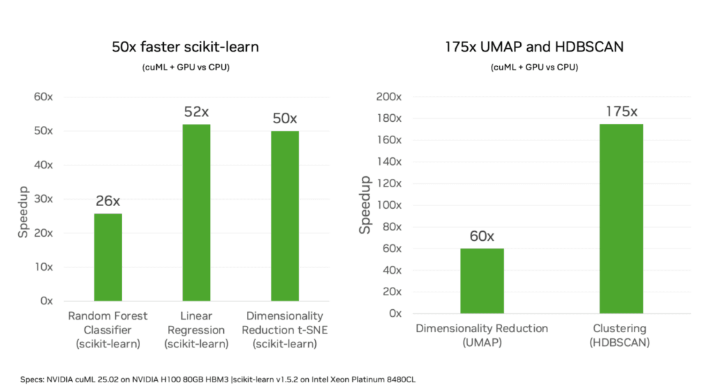
Source: https://developer.nvidia.com/
And the best part? You don’t need to refactor your code. Just load the extension, keep using the familiar scikit-learn API, and enjoy GPU-accelerated results.
Quote from NVIDIA
“Users can reduce training time from hours on CPUs to mere seconds on GPUs with zero code change.”
— Siddharth Sharma, Nick Becker, Brian Tepera, and Dante Gama Dessavre, NVIDIA
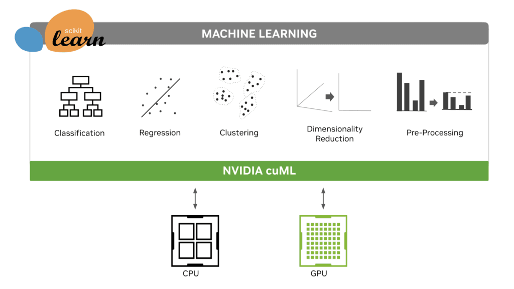
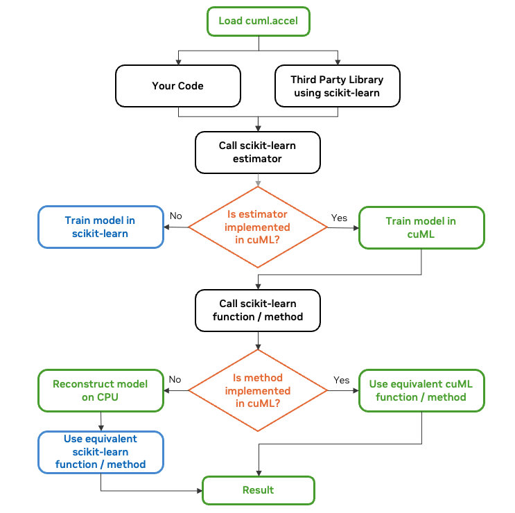
How Does Zero Code Change Acceleration Work?
Source: https://developer.nvidia.com/
- The Magic Line
By inserting"%load_ext cuml.accel"at the top of your notebook—or usingpython -m cuml.accel script.pyfor standalone scripts—cuML intercepts your scikit-learn calls under the hood. - GPU Where Possible, CPU Where Needed
If cuML supports a particular scikit-learn function (like RandomForestClassifier), computations automatically run on the GPU. If not, it falls back to the CPU seamlessly. - Transparent Data Transfers
When data moves between the CPU and GPU, cuML manages the process so you don’t have to worry about memory allocations or conversions. You keep writing ordinary Python code.
Key takeaway: You don’t have to rewrite your code or learn an entirely new API. It’s the scikit-learn you know and love—just faster.
Real-World Speedups
One of the most exciting aspects of cuML is its performance on algorithms that traditionally take a long time on CPUs. Below is a snapshot of how much time we saved in our test:
| Algorithm | Dataset | CPU Time (s) | GPU Time (s) | Speedup |
|---|---|---|---|---|
| Random Forest | Covertype (580k x 54 features) | 87.60 | 8.79 | ~10x |
| HDBSCAN | Synthetic (100k x 100 features) | 1,093.78 | 5.06 | ~216x |
| UMAP | MNIST (50k x 784 features) | 71.31 | 5.39 | ~13x |
This table says it all: faster training, quicker experimentation, and more time to focus on what matters—insights rather than waiting.
Why GPU Acceleration Rocks
- Parallel Processing
GPUs excel at handling thousands of operations simultaneously, making tasks like distance calculations and matrix operations lightning-fast. - Bigger, More Complex Models
With speed improvements of 50x or more, you can comfortably explore larger datasets, conduct extensive hyperparameter searches, and iterate on more sophisticated models. - Easy Integration
If scikit-learn is already part of your workflow, you won’t miss a beat. Import your libraries, add the cuML extension, and you’re off to the races.
Quick Tips for a Smooth Experience
Tip:
To see your GPU usage really shine, use larger datasets or highly iterative algorithms. Small datasets or trivial operations might not show significant speedups.
- Stay on the GPU
Preprocess and train on the GPU to minimize data transfers between host (CPU) and device (GPU). Use libraries like cuDF (a GPU-accelerated drop-in for pandas) for data manipulation. - Watch for Unsupported Features
cuML supports many (but not all) scikit-learn methods. If you call a method that’s not yet implemented, it automatically runs on the CPU. No errors or warnings—just a seamless fallback. - Be Prepared for Slight Numerical Differences
Parallel operations sometimes yield slightly different floating-point accumulations compared to serial CPU code. Don’t be alarmed; these differences are usually trivial.
Known Gotchas
Warning:
Once cuML acceleration is loaded, it keeps intercepting scikit-learn. If you want to measure CPU performance in the same notebook session, you typically need to restart your runtime and not load cuml.accel until after you gather CPU benchmarks.
- String or Categorical Data: Ensure data is numeric. Encode categorical features before passing them to scikit-learn with cuML enabled.
- Memory Constraints: Although cuML can use unified memory to help, extremely large datasets may still exceed GPU memory. Monitor resource usage.
Use Cases That Benefit the Most
- High-Dimensional Data: Techniques like UMAP or t-SNE can become unbearably slow on CPUs as dimensions grow. On GPUs, they can feel almost real-time by comparison.
- Complex Clustering: Algorithms like HDBSCAN can now handle large volumes of data quickly, unlocking deeper insights into unlabeled datasets.
- Rapid Prototyping & Hyperparameter Tuning: Grid searches or random searches for model selection become far more feasible when each model trains in a fraction of the time.
Hands-On GPU Acceleration Demo
Here’s a short introduction you can place under that heading:
In the following video, you’ll see exactly how cuML intercepts your scikit-learn, UMAP, and HDBSCAN calls in real time—without changing a single line of your model code. Watch as we demonstrate data loading, model training, and performance benchmarks in a live session, showcasing the dramatic speedups made possible by NVIDIA GPUs.
Code
Random Forest Classification
In this section, we’ll train and time a Random Forest classifier on the Covertype dataset to compare CPU-based scikit-learn performance with GPU-accelerated cuML. We use the exact same code parameters—just swap in the cuML accelerator for a massive speed boost.
Code:
import time
import pandas as pd
import numpy as np
import matplotlib.pyplot as plt

from sklearn.datasets import fetch_covtype
from sklearn.model_selection import train_test_split
from sklearn.metrics import accuracy_score
from sklearn.ensemble import RandomForestClassifier

# Utility function to measure execution time
def time_execution(func, *args, **kwargs):
    start_time = time.time()
    result = func(*args, **kwargs)
    end_time = time.time()
    return result, end_time - start_time

def main():
    print("\n" + "="*50)
    print("PART 1: Random Forest Classification (Full Dataset)")
    print("="*50)

    # Load the entire Covertype dataset
    print("Loading full Covertype dataset...")
    data = fetch_covtype()
    X, y = data.data, data.target
    print(f"Full dataset shape: {X.shape}")

    # Split the data
    X_train, X_test, y_train, y_test = train_test_split(
        X, y, test_size=0.2, random_state=42
    )

    # ===========================================
    # First: Run with standard scikit-learn
    # ===========================================
    print("\nRunning with standard scikit-learn:")
    rf_sklearn = RandomForestClassifier(
        n_estimators=100, max_depth=20, random_state=42, n_jobs=-1
    )
    _, sklearn_time = time_execution(rf_sklearn.fit, X_train, y_train)
    print(f"Training time with scikit-learn: {sklearn_time:.2f} seconds")

    test_subset = 10000
    sklearn_preds, sklearn_pred_time = time_execution(
        rf_sklearn.predict, X_test[:test_subset]
    )
    print(f"Prediction time with scikit-learn (on {test_subset} samples): {sklearn_pred_time:.2f} seconds")
    sklearn_accuracy = accuracy_score(y_test[:test_subset], sklearn_preds)
    print(f"Accuracy with scikit-learn: {sklearn_accuracy:.4f}")

    # ===========================================
    # Now: Run with cuML acceleration
    # ===========================================
    print("\nRunning with cuML acceleration:")
    # NOTE: In a .py script, use:
    #       python -m cuml.accel random_forest_test.py
    #       to enable the accelerator.
    from sklearn.ensemble import RandomForestClassifier  # re-import after accel

    rf_cuml = RandomForestClassifier(
        n_estimators=100, max_depth=20, random_state=42, n_jobs=-1
    )
    _, cuml_time = time_execution(rf_cuml.fit, X_train, y_train)
    print(f"Training time with cuML: {cuml_time:.2f} seconds")

    cuml_preds, cuml_pred_time = time_execution(
        rf_cuml.predict, X_test[:test_subset]
    )
    print(f"Prediction time with cuML (on {test_subset} samples): {cuml_pred_time:.2f} seconds")
    cuml_accuracy = accuracy_score(y_test[:test_subset], cuml_preds)
    print(f"Accuracy with cuML: {cuml_accuracy:.4f}")

    # Calculate speedup
    rf_speedup = sklearn_time / cuml_time if cuml_time else 0
    rf_pred_speedup = sklearn_pred_time / cuml_pred_time if cuml_pred_time else 0
    print(f"\nSpeedup for Random Forest training: {rf_speedup:.2f}x")
    print(f"Speedup for Random Forest prediction: {rf_pred_speedup:.2f}x")

    # Visualize timing
    labels = ['scikit-learn', 'cuML (GPU)']
    train_times = [sklearn_time, cuml_time]
    pred_times = [sklearn_pred_time, cuml_pred_time]

    plt.figure(figsize=(12, 5))

    # Training time comparison
    plt.subplot(1, 2, 1)
    plt.bar(labels, train_times)
    plt.title('Random Forest Training Time (seconds)')
    plt.ylabel('Time (seconds)')
    for i, v in enumerate(train_times):
        plt.text(i, v + max(train_times)*0.05, f"{v:.2f}s", ha='center')

    # Prediction time comparison
    plt.subplot(1, 2, 2)
    plt.bar(labels, pred_times)
    plt.title('Random Forest Prediction Time (seconds)')
    plt.ylabel('Time (seconds)')
    for i, v in enumerate(pred_times):
        plt.text(i, v + max(pred_times)*0.05, f"{v:.2f}s", ha='center')

    plt.tight_layout()
    plt.savefig('rf_timing_comparison_large.png')
    plt.show()

if __name__ == "__main__":
    main()
Output & Results
==================================================
PART 1: Random Forest Classification (Full Dataset)
==================================================
Loading full Covertype dataset...
Full dataset shape: (581012, 54)

Running with standard scikit-learn:
Training time with scikit-learn: 87.60 seconds
Prediction time with scikit-learn (on 10000 samples): 0.18 seconds
Accuracy with scikit-learn: 0.8920

Running with cuML acceleration:
...
Training time with cuML: 8.79 seconds
Prediction time with cuML (on 10000 samples): 0.33 seconds
Accuracy with cuML: 0.7387

Speedup for Random Forest training: 9.97x
Speedup for Random Forest prediction: 0.54x
Here we see nearly 10x faster training on the GPU, though prediction speed shows a slight slowdown in this particular test (which can happen with small batch sizes). The GPU-accelerated approach still offers huge advantages when training times are the bottleneck.
HDBSCAN Clustering
Code:
import time
import numpy as np
import matplotlib.pyplot as plt

from sklearn.datasets import make_blobs
from sklearn.metrics import silhouette_score

# Utility function to measure execution time
def time_execution(func, *args, **kwargs):
    start_time = time.time()
    result = func(*args, **kwargs)
    end_time = time.time()
    return result, end_time - start_time

def main():
    print("\n" + "="*50)
    print("PART 2: HDBSCAN Clustering (Larger Dataset)")
    print("="*50)

    # Generate a larger synthetic dataset
    n_samples = 100000
    n_features = 100
    print(f"Generating larger dataset with {n_samples} samples and {n_features} features...")

    X_clusters, y_true = make_blobs(
        n_samples=n_samples,
        n_features=n_features,
        centers=10,
        cluster_std=[1.0, 2.0, 0.5, 3.0, 1.5, 1.2, 2.5, 0.8, 1.7, 2.2],
        random_state=42
    )

    # ===========================================
    # First: Run with standard HDBSCAN
    # ===========================================
    print("\nRunning with standard HDBSCAN:")
    import hdbscan

    clusterer_std = hdbscan.HDBSCAN(min_cluster_size=100, min_samples=10)
    _, hdbscan_time = time_execution(clusterer_std.fit, X_clusters)
    print(f"Clustering time with standard HDBSCAN: {hdbscan_time:.2f} seconds")

    # Evaluate clustering quality (using a sample for silhouette score)
    sample_size = min(10000, len(X_clusters))
    indices = np.random.choice(len(X_clusters), sample_size, replace=False)
    if len(np.unique(clusterer_std.labels_)) > 1:
        silhouette_std = silhouette_score(X_clusters[indices], clusterer_std.labels_[indices])
    else:
        silhouette_std = 0
    print(f"Silhouette score with standard HDBSCAN (on {sample_size} samples): {silhouette_std:.4f}")
    num_clusters_std = len(np.unique(clusterer_std.labels_)) - (1 if -1 in clusterer_std.labels_ else 0)
    print(f"Number of clusters found: {num_clusters_std}")

    # ===========================================
    # Now: Run with cuML acceleration
    # ===========================================
    print("\nRunning with cuML acceleration:")
    # NOTE: In a .py script, use:
    #       python -m cuml.accel hdbscan_test.py
    import hdbscan  # re-import after accel

    clusterer_cuml = hdbscan.HDBSCAN(min_cluster_size=100, min_samples=10)
    _, hdbscan_cuml_time = time_execution(clusterer_cuml.fit, X_clusters)
    print(f"Clustering time with cuML HDBSCAN: {hdbscan_cuml_time:.2f} seconds")

    if len(np.unique(clusterer_cuml.labels_)) > 1:
        silhouette_cuml = silhouette_score(X_clusters[indices], clusterer_cuml.labels_[indices])
    else:
        silhouette_cuml = 0
    print(f"Silhouette score with cuML HDBSCAN (on {sample_size} samples): {silhouette_cuml:.4f}")
    num_clusters_cuml = len(np.unique(clusterer_cuml.labels_)) - (1 if -1 in clusterer_cuml.labels_ else 0)
    print(f"Number of clusters found: {num_clusters_cuml}")

    # Calculate speedup
    hdbscan_speedup = hdbscan_time / hdbscan_cuml_time if hdbscan_cuml_time > 0 else 0
    print(f"\nSpeedup for HDBSCAN clustering: {hdbscan_speedup:.2f}x")

    # Visualize timing
    labels = ['HDBSCAN (CPU)', 'HDBSCAN with cuML (GPU)']
    cluster_times = [hdbscan_time, hdbscan_cuml_time]

    plt.figure(figsize=(10, 6))
    plt.bar(labels, cluster_times)
    plt.title('HDBSCAN Clustering Time (seconds)')
    plt.ylabel('Time (seconds)')
    for i, v in enumerate(cluster_times):
        plt.text(i, v + max(cluster_times)*0.05, f"{v:.2f}s", ha='center')

    plt.tight_layout()
    plt.savefig('hdbscan_timing_comparison_large.png')
    plt.show()

if __name__ == "__main__":
    main()
Output & Results
==================================================
PART 2: HDBSCAN Clustering (Larger Dataset)
==================================================
Generating larger dataset with 100000 samples and 100 features...

Running with standard HDBSCAN:
Clustering time with standard HDBSCAN: 1093.78 seconds
Silhouette score with standard HDBSCAN (on 10000 samples): 0.7175
Number of clusters found: 10

Running with cuML acceleration:
Clustering time with cuML HDBSCAN: 5.06 seconds
Silhouette score with cuML HDBSCAN (on 10000 samples): 0.7175
Number of clusters found: 10

Speedup for HDBSCAN clustering: 216.36x
Here, HDBSCAN saw a jaw-dropping 216x speedup. Notably, the silhouette score is the same, indicating the clusters discovered by CPU and GPU versions are effectively identical in quality.
UMAP Dimensionality Reduction
Finally, we apply the UMAP algorithm to reduce a 50,000-sample MNIST dataset (784 features each) down to 2D. UMAP can be computationally heavy, so it’s a prime example of how GPU acceleration can drastically cut processing times.
Code:
import time
import numpy as np
import matplotlib.pyplot as plt

from sklearn.datasets import fetch_openml
from sklearn.preprocessing import StandardScaler

# Utility function to measure execution time
def time_execution(func, *args, **kwargs):
    start_time = time.time()
    result = func(*args, **kwargs)
    end_time = time.time()
    return result, end_time - start_time

def main():
    print("\n" + "="*50)
    print("PART 3: UMAP Dimensionality Reduction (Larger Dataset)")
    print("="*50)

    # Load a larger subset of MNIST
    print("Loading larger MNIST dataset...")
    X_mnist, y_mnist = fetch_openml('mnist_784', version=1, return_X_y=True, parser='auto')
    X_mnist = X_mnist.to_numpy()[:50000]
    y_mnist = y_mnist.to_numpy()[:50000]

    scaler = StandardScaler()
    X_mnist_scaled = scaler.fit_transform(X_mnist)
    print(f"MNIST subset shape: {X_mnist_scaled.shape}")

    # ===========================================
    # First: Run with standard UMAP
    # ===========================================
    print("\nRunning with standard UMAP:")
    import umap

    umap_std = umap.UMAP(
        n_neighbors=15, min_dist=0.1, n_components=2, random_state=42
    )
    (X_umap_std, ), umap_time = time_execution(
        umap_std.fit_transform, X_mnist_scaled
    )
    print(f"UMAP time with standard library: {umap_time:.2f} seconds")

    # ===========================================
    # Now: Run with cuML acceleration
    # ===========================================
    print("\nRunning with cuML acceleration:")
    # NOTE: In a .py script, use:
    #       python -m cuml.accel umap_test.py
    import umap  # re-import after accel

    umap_cuml = umap.UMAP(
        n_neighbors=15, min_dist=0.1, n_components=2, random_state=42
    )
    (X_umap_cuml, ), umap_cuml_time = time_execution(
        umap_cuml.fit_transform, X_mnist_scaled
    )
    print(f"UMAP time with cuML: {umap_cuml_time:.2f} seconds")

    # Calculate speedup
    umap_speedup = umap_time / umap_cuml_time if umap_cuml_time else 0
    print(f"\nSpeedup for UMAP dimensionality reduction: {umap_speedup:.2f}x")

    # Visualize timing
    labels = ['UMAP (CPU)', 'UMAP with cuML (GPU)']
    umap_times = [umap_time, umap_cuml_time]

    plt.figure(figsize=(10, 6))
    plt.bar(labels, umap_times)
    plt.title('UMAP Execution Time (seconds)')
    plt.ylabel('Time (seconds)')
    for i, v in enumerate(umap_times):
        plt.text(i, v + max(umap_times)*0.05, f"{v:.2f}s", ha='center')

    plt.tight_layout()
    plt.savefig('umap_timing_comparison_large.png')
    plt.show()

if __name__ == "__main__":
    main()
Output & Results
==================================================
PART 3: UMAP Dimensionality Reduction (Larger Dataset)
==================================================
Loading larger MNIST dataset...
MNIST subset shape: (50000, 784)

Running with standard UMAP:
UMAP time with standard library: 71.31 seconds

Running with cuML acceleration:
UMAP time with cuML: 5.39 seconds

Speedup for UMAP dimensionality reduction: 13.24x
With UMAP, we enjoyed an impressive 13x speed boost on a modest T4 GPU. More advanced hardware (like NVIDIA A100 or H100) would see even bigger gains.
How to Run These Tests
- Install Dependencies
Make sure you have the required packages installed:scikit-learn,cuml,hdbscan,umap-learn,matplotlib, and so forth. - Enable cuML Acceleration
In a.pyscript, use the syntax:python -m cuml.accel random_forest_test.pyto ensure the cuML accelerator is loaded beforescikit-learnor other libraries. - Inspect the Outputs
Each script prints timing information, speedups, and (where applicable) metrics like accuracy and silhouette scores. You’ll also see bar charts in.pngfiles comparing CPU vs GPU times.
Feel free to adapt these examples to your own datasets and pipelines. With NVIDIA cuML, virtually any scikit-learn pipeline can run faster—all while keeping your code unchanged.
Conclusion
NVIDIA cuML’s zero code change acceleration stands out as a genuinely game-changing leap in the Python machine learning ecosystem. By adopting a friendly one-line extension, data scientists and ML engineers get an enormous performance boost—often over 50x—without the usual headache of rewriting perfectly good scikit-learn code.
If you’re juggling large datasets, tuning hyperparameters, or just sick of endless wait times, this is your golden ticket to faster, more efficient workflows. So, go ahead—load the extension, run your code, and watch your productivity soar.