I. INTRODUCTION
Definition and Overview of Recurrent Neural Networks
Recurrent Neural Networks, or RNNs for short, are a special kind of neural network. Imagine a group of friends playing a game of whisper down the lane. Each friend hears a message, remembers it for a bit, and then passes it on to the next friend. An RNN works a lot like this game. It can remember information for a short time and use it to help make decisions.
Unlike a normal neural network, which only looks at present inputs to make decisions, RNNs also consider what they’ve learned from past inputs. This ‘remembering’ power is what makes them ‘recurrent’. They’re a bit like time travelers in the deep learning universe because they can remember and use information from the past.
Why Recurrent Neural Networks are Crucial in Deep Learning
RNNs play a very important role in deep learning. They’re especially good at understanding sequences – like a series of words in a sentence or the notes in a piece of music. This makes them really useful for tasks like understanding language, predicting what note might come next in a song, or even helping self-driving cars make decisions based on past events.
Let’s say you’re reading a book. You understand the meaning of each sentence because you remember the sentences you’ve read before. RNNs can do something similar, and that’s why they’re so important in deep learning.
II. BACKGROUND INFORMATION
Recap of Feedforward Networks and Their Limitations
Before we talk more about RNNs, let’s take a step back and remember what we know about feedforward neural networks. These are the most basic type of neural networks. They’re a bit like a factory production line. Information enters at one end, gets processed in a single direction, and then comes out as a decision at the other end.
But feedforward networks have a big limitation: they can’t remember anything from the past. They just look at the present input to make their decision. This is like trying to understand a book by reading just one sentence – it’s quite hard!
The Emergence of Recurrent Neural Networks
That’s where RNNs come in. Scientists thought, “Hey, what if our neural networks could remember things from the past? That could help them make better decisions!” And so, RNNs were born. They introduced a loop in the network that allowed information to be passed from one step in the sequence to the next, helping the network to ‘remember’ past information.
The Role of RNNs in Machine Learning and Artificial Intelligence
Since then, RNNs have played a big role in machine learning and artificial intelligence. They’re used in lots of different tasks that need an understanding of sequences. This includes things like language translation, speech recognition, and even predicting the stock market. If there’s a sequence to understand, an RNN can probably help!
III. DISSECTING THE STRUCTURE OF RNNs
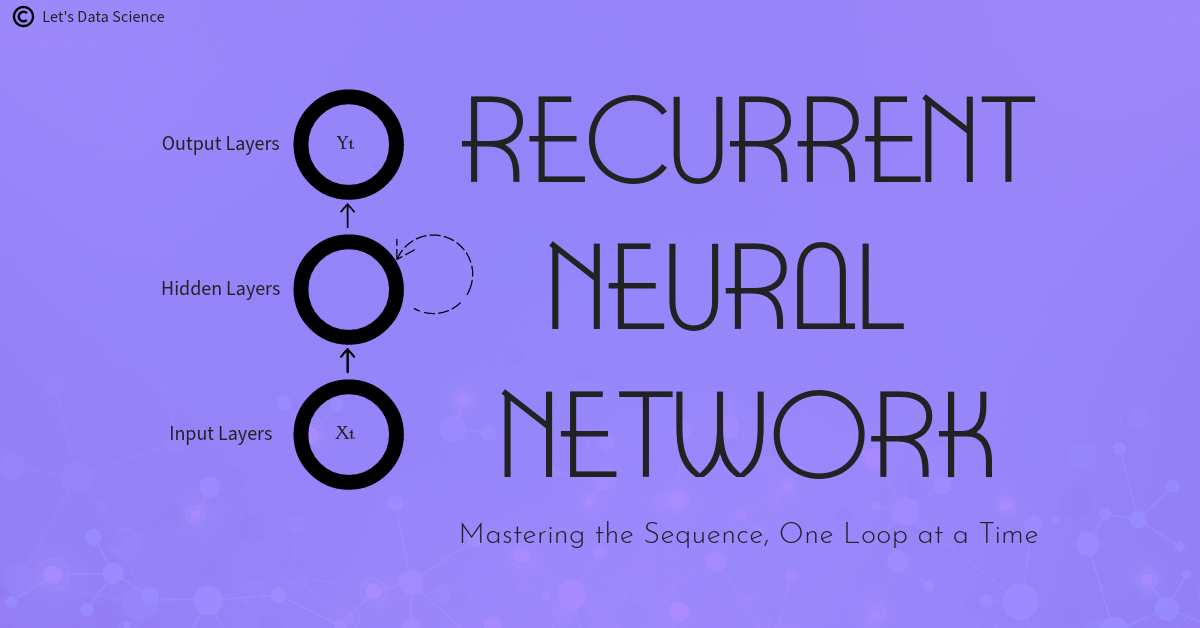
Understanding the Input Layer
Think of the input layer of an RNN as the gatekeeper or the front door. It’s where all the information first enters the network. Just like you’d enter your house through the front door, information enters an RNN through the input layer. This could be any kind of information – words from a sentence notes from a song, or even numbers from a stock market.
Imagine your friend telling you a sentence, “The cat is on the mat.” To understand it, you need to remember each word in the order your friend tells you. Each word in this sentence – “The”, “cat”, “is”, “on”, “the”, “mat” – enters the RNN one after the other through the input layer.
The Hidden Magic: Hidden Layer in RNNs
After entering through the input layer, information moves to the hidden layer. This is where the real magic happens! You can imagine this as a magic box where information from the past and the present come together.
Remember how we said RNNs can remember things? Well, the hidden layer is the part of the RNN that does this. It takes the present input (like “mat” from our sentence) and combines it with what it remembers from the past (like “The”, “cat”, “is”, “on”, “the”).
Interpreting the Output Layer
The output layer of an RNN is like the exit door. It’s where the RNN makes a decision based on the information it’s received and remembered.
Continuing with our sentence example, once the RNN has processed the entire sentence, it might make a decision about what the sentence means. Maybe it decides the sentence is talking about a cat on a mat!
Unfolding the RNN: A Step-by-Step Perspective
Understanding an RNN can be tricky, so let’s take it slow and look at what happens step by step.
- First, our RNN gets an input, like “The” from our sentence. It sends this to the magic box (the hidden layer).
- The magic box looks at the input, “The”, and also remembers what it learned from the past. Since this is the first word, it doesn’t remember anything yet!
- The magic box then sends its understanding of “The” to the output layer. The output layer makes a decision based on this and also sends some information back to the magic box to be remembered for later.
- Then, the next word, “cat”, enters the input layer. This process repeats until all the words in the sentence have been processed.
So you see, at every step, the RNN is remembering what it learned from the previous steps, which helps it understand the whole sentence.
Neurons, Weights, and Biases in RNNs
An RNN, like all neural networks, is made up of lots of little parts called neurons. These neurons are like tiny decision-makers. They each look at a bit of information, make a decision about it, and pass that decision on to the next neuron.
Each neuron also has something called weights and biases. These are like the neuron’s personal rulebook that it uses to make decisions. The weights tell the neuron how important each bit of information is, and the bias helps the neuron make a final decision.
So, in a way, each neuron in an RNN is a tiny decision-maker. They all work together to help the RNN understand and remember information.
IV. THE LEARNING PROCESS OF RNNs: FORWARD PROPAGATION, LOSS FUNCTION, AND BACKPROPAGATION
Forward Propagation in RNNs: Passing the Information
Let’s imagine that you are playing a game of catch. You throw the ball, your friend catches it and then they throw it back. This is a bit like how information travels through an RNN. It’s called “forward propagation”.
When the RNN gets an input, like “The” from our sentence, it throws this information into the magic box (the hidden layer). The magic box catches the information, combines it with what it remembers from the past, and then throws its understanding to the exit door (the output layer).
This keeps happening until all the inputs have been processed. So, in a way, forward propagation is like a game of catch between the input layer, the magic box, and the output layer!
Understanding Loss Function in RNNs
Now, imagine you’re learning to play a new game. At first, you might make a lot of mistakes. But as you keep playing, you learn from those mistakes and get better. This is exactly what happens in an RNN.
The RNN tries to predict the meaning of a sentence, like “The cat is on the mat”. But it might make mistakes. Maybe it thinks the sentence is about a dog, not a cat! We can measure how big these mistakes are using something called a “loss function”.
The loss function is like a rulebook that says how bad the RNN’s mistakes are. If the RNN predicts something very wrong, the loss function gives a big number. If the RNN predicts something pretty close to the right answer, the loss function gives a small number. So, the loss function helps us understand how well the RNN is learning.
Backpropagation Through Time (BPTT): Learning from Mistakes
Remember when we said the RNN learns from its mistakes? This is where “backpropagation through time”, or BPTT for short, comes in.
Think of BPTT as a time machine. It allows the RNN to go back in time to when it made a mistake, understand what went wrong, and then update its rulebook (the weights and biases) to avoid that mistake in the future. It’s like getting a chance to replay a round in a game after knowing the correct moves.
So BPTT is how an RNN learns. It keeps going back in time, learning from its mistakes, until it gets better and better at understanding sentences, songs, or whatever information it’s learning from!
Role of the Learning Rate in RNNs
Lastly, let’s talk about the learning rate. The learning rate is like a teacher guiding the RNN’s learning process.
Let’s say the RNN made a big mistake and the loss function gave a big number. The RNN needs to learn from this mistake and update its rulebook. But how much should it change the rulebook? A little bit? A lot? This is what the learning rate decides.
A big learning rate means the RNN changes its rulebook a lot after every mistake. A small learning rate means the RNN changes its rulebook just a little bit. The right learning rate can help the RNN learn efficiently from its mistakes. So, it’s a very important part of the learning process!
And that’s it! That’s how RNNs learn: they pass information forward, measure their mistakes with the loss function, learn from their mistakes with BPTT, and use the learning rate to guide their learning. It’s a lot like learning to play a new game!
V. MATHEMATICAL UNDERSTANDINGS OF RNNs
Mathematical Representation of Forward Propagation in RNNs
Let’s think of forward propagation like a fun game of treasure hunting. Each neuron is a clue and each clue leads you closer to the treasure. But instead of a map, we have a mathematical equation to guide us.
Let’s start with our first clue, which is the input. Let’s say we’re trying to understand the sentence, “The cat is on the mat”. We’ll represent each word in the sentence with a number. For example, we can say “The” is 1, “cat” is 2, and so on.
Now, remember our magic box (the hidden layer)? It takes our clue (the input) and combines it with a hint from the previous clue (what it remembers from the past). We can write this down as:
h_t = f(W * x_t + U * h_(t-1) + b)In this equation:
- “h_t” represents the hint from the magic box at the current clue (t).
- “f” is the function that the magic box uses to combine the current clue and the hint from the past clue.
- “W” and “U” are like the magic box’s secret decoder for the clue. They tell the magic box how important each part of the clue is.
- “x_t” is our current clue (input), and “h_(t-1)” is the hint from the previous clue.
- “b” is the magic box’s guess before it even looks at the clue. It’s a bit like a starting point.
So, the magic box (hidden layer) uses this equation to find the next clue. This keeps happening until we find the treasure (reach the output)!
Calculating the Loss Function: A Mathematical Perspective
Remember how we measure how far we are from the treasure (the correct answer)? That’s the loss function. The loss function is like a measuring tape that tells us how far off we are from the treasure.
We can write down the loss function like this:
L = 1/2 * (y - y')^2In this equation:
- “L” is the length of the measuring tape, which is our loss.
- “y” is the location of the treasure (the correct answer).
- “y'” is where we are right now (the RNN’s prediction).
- The “^2” means we’re squaring the difference between the correct answer and our prediction.
If our prediction is very wrong, this number becomes big. If our prediction is pretty close, this number is small. So, this equation helps us understand how far we are from the treasure (the correct answer) and how much we need to adjust our course.
Demystifying Backpropagation Through Time (BPTT)
Backpropagation Through Time (BPTT) is our time machine that lets us go back and correct our mistakes. It’s a bit complicated, but let’s break it down.
BPTT can be written as:
dW = dL/dh_t * dh_t/dWIn this equation:
- “dW” is how much we want to change our secret decoder (the weights).
- “dL/dh_t” is how the length of the measuring tape (loss) changes when we change our hint from the magic box.
- “dh_t/dW” is how the hint from the magic box changes when we change our secret decoder.
So, the time machine uses this equation to figure out how much to change our secret decoder (weights) to avoid the same mistake in the future.
Understanding the Impact of Learning Rate: A Mathematical Insight
Lastly, we have our teacher, the learning rate. It guides how much we should change our secret decoder (weights) after every mistake.
Let’s say we figured out we need to change our decoder by a certain amount (dW). The teacher (learning rate) tells us to adjust this change. We can write this as:
W_new = W_old - lr * dWIn this equation:
- “W_new” is our updated secret decoder.
- “W_old” is our old secret decoder.
- “lr” is our teacher (learning rate).
- “dW” is the change we want to make to our decoder.
If the teacher is strict (big learning rate), we change our decoder a lot. If the teacher is lenient (small learning rate), we change our decoder just a little bit.
So that’s it! With these mathematical equations, we’ve decoded how an RNN learns. But remember, learning is a journey. So, let’s keep going and see how we can make our RNN even better in the next section!
VI. OPTIMIZATION AND REGULARIZATION IN RNNs
Optimizing RNNs: SGD, Adam, RMSprop
We’ve already learnt how an RNN can learn and correct its mistakes. But wouldn’t it be amazing if we could help our RNN learn even faster and better? Well, we can do that with something called “optimizers”!
Let’s think of our RNN as a hiker trying to find the top of a mountain (the best answer). The optimizers are like the hiker’s GPS, guiding the hiker to the top in the quickest and easiest way possible.
One of these GPS systems is called Stochastic Gradient Descent or SGD for short. SGD looks around and finds the steepest path up the mountain. Then, it tells the hiker to go that way. But sometimes, the steepest path isn’t always the fastest or easiest one.
That’s why we have other GPS systems like Adam and RMSprop. These GPS systems are a bit smarter. They look around, remember the paths they’ve tried before, and make a more informed decision about the best path to take. So, these optimizers help the hiker (our RNN) reach the top of the mountain (the best answer) in a smarter and quicker way!
Regularization Techniques: Dropout, L2 Regularization, and Sequence Masking
Now, let’s say our hiker has become really good at climbing this particular mountain. But what if we take our hiker to a new mountain? Will they still be good at climbing? We want our hiker to be good at climbing any mountain, not just this one. This is where “regularization” techniques come in.
Regularization techniques are like different training exercises to make our hiker stronger and more versatile. One of these exercises is called “Dropout”. Dropout randomly leaves out some neurons during training. It’s like asking our hiker to climb the mountain with one hand tied behind their back. This way, our hiker learns to not rely too much on any one path and becomes more versatile.
Another exercise is called “L2 Regularization”. It penalizes the hiker if they rely too much on a specific path. It’s like adding an extra weight to the hiker’s backpack every time they take a specific path. This way, the hiker learns to find different paths to the top.
Lastly, we have “Sequence Masking”. This is like asking the hiker to climb the mountain blindfolded for a few steps. It helps the hiker learn to remember and use information from the past effectively. This is especially helpful when dealing with sequence data like sentences or songs.
So, these regularization techniques help our hiker (RNN) become stronger, more versatile, and ready to climb any mountain (solve any problem)!
Importance of Parameter Initialization
Remember how we talked about the secret decoder (weights) in our RNN? Well, before our RNN starts learning, these weights are set to initial values. You can think of it as setting the compass before starting a journey.
Choosing the right initial values for our weights (or setting the compass in the right direction) can help our RNN start learning in a good way. This can speed up the learning process and help the RNN reach a better answer. It’s a bit like giving our hiker a head start in their journey up the mountain.
So, parameter initialization is a very important step in our RNN’s journey to learning. It sets the stage for everything that follows!
So, there you have it! Optimization, regularization, and parameter initialization are some of the ways we can help our RNN learn better and faster.
VII. DIVE INTO VARIANTS OF RNNs
Exploring LSTM: Long Short-Term Memory Networks
Remember our magic box (the hidden layer in RNNs) we’ve been talking about? Well, Long Short-Term Memory Networks or LSTMs for short, are like an upgraded version of this magic box!
You see, standard RNNs have a slight problem. They are forgetful. If you tell them a long story, they might forget the beginning of the story by the time they get to the end. This can be a problem, especially when the beginning of the story is important for understanding the end!
LSTMs solve this problem by having a special trick. They carry a “memory” from the beginning of the story to the end. Imagine it like this: the LSTM is a person reading a book with a magical bookmark. This bookmark not only marks the page but also stores important information from the previous pages. So, when our LSTM person comes across something important, they can refer to this magical bookmark and remember the key details!
This makes LSTMs really good at understanding things like sentences, where the meaning of each word can depend on the words that came before it!
Understanding GRU: Gated Recurrent Units
Gated Recurrent Units or GRUs for short, are another type of magic box (hidden layer in RNNs). They are a bit like LSTMs but with a slight twist.
You see, LSTMs are like a person with a magical bookmark, but GRUs are like a person with a magical highlighter. Instead of storing important information from the previous pages like the LSTM’s bookmark, the GRU’s highlighter just highlights the important parts. This way, the GRU person only focuses on the highlighted parts and can ignore the rest!
This makes GRUs a bit simpler and faster than LSTMs. They are really good when you have a lot of data and you want to train your RNN quickly!
Bidirectional RNNs: Looking Forward and Backward
Last but not least, let’s talk about Bidirectional RNNs. These are a bit different from LSTMs and GRUs. Instead of just reading the book from start to finish like LSTMs and GRUs, Bidirectional RNNs read the book from both ends!
Imagine it like this: Bidirectional RNN is a person with two magical bookmarks. One bookmark starts from the beginning of the book and moves forward, while the other starts from the end of the book and moves backward. This way, our Bidirectional RNN person can understand the story from both ends!
This makes Bidirectional RNNs really good at understanding things like sentences, where the meaning of a word can depend on the words that came before and after it!
And that’s it! These are the different types of RNNs. Each one of them has their own special skills and can be used for different tasks.
VIII. BUILDING AN RNN: A PRACTICAL EXAMPLE
Identifying a Real-world Problem that Can be Solved Using RNN
Now that we’ve learned all about RNNs, it’s time to use one to solve a real-world problem. Remember how we said that RNNs are really good at understanding things like sentences? Well, we’re going to use an RNN to do just that!
Let’s say we have a bunch of movie reviews and we want to know if they’re positive or negative. This is a task called “sentiment analysis”, and it’s something that RNNs are really good at. So, we’re going to build an RNN that reads movie reviews and tells us if they’re thumbs up or thumbs down!
Implementing an RNN using Python and TensorFlow/Keras
To build our RNN, we’re going to use Python, which is a programming language that’s really good for things like machine learning. And we’re going to use a library called TensorFlow, which has a lot of tools that make building neural networks easier. Specifically, we’ll use Keras, which is part of TensorFlow that’s even more focused on neural networks.
First, we need to import the tools we’re going to use:
import tensorflow as tf
from tensorflow.keras.models import Sequential
from tensorflow.keras.layers import Embedding, SimpleRNN, Dense
Next, we need to build our RNN. Remember how our RNN is like a hiker climbing a mountain? Well, building our RNN is like giving our hikers the tools they need for their journey. We’re going to give our hiker (our RNN) three tools: an Embedding layer, a SimpleRNN layer, and a Dense layer.
model = Sequential()
model.add(Embedding(10000, 32)) # The Embedding layer
model.add(SimpleRNN(32)) # The SimpleRNN layer
model.add(Dense(1, activation='sigmoid')) # The Dense layer
The Embedding layer is like a dictionary. It turns words into numbers that our RNN can understand. The SimpleRNN layer is our magic box. It takes the numbers from the Embedding layer and uses them to understand the sentence. The Dense layer is like a judge. It takes the understanding from the SimpleRNN layer and decides if the review is positive or negative.
After building our model, we need to compile it. This is like telling our hiker the rules of their journey. We need to tell our model what optimizer to use, what loss function to use, and what metrics to use.
model.compile(optimizer='rmsprop', loss='binary_crossentropy', metrics=['acc'])
Now, our model is ready to start learning!
Walkthrough of Code and Interpretation of Results
Once our RNN is built and compiled, we need to train it. This is where our hiker starts climbing the mountain. To train our RNN, we’re going to use our movie reviews and their labels (thumbs up or thumbs down). We’ll give these to our RNN and let it learn from them.
history = model.fit(input_train, y_train, epochs=10, batch_size=128, validation_split=0.2)
After training, our RNN will have learned to understand movie reviews! We can check how well it’s doing by looking at the accuracy on the training data and the validation data.
import matplotlib.pyplot as plt

acc = history.history['acc']
val_acc = history.history['val_acc']

plt.plot(acc, label='Training acc')
plt.plot(val_acc, label='Validation acc')
plt.title('Training and validation accuracy')
plt.legend()
plt.show()
The blue line shows how well our RNN is doing on the training data, and the orange line shows how well it’s doing on the validation data. If our RNN is learning well, both lines should be going up!
And that’s how we build an RNN! It might seem complicated at first, but once you get the hang of it, it’s just like guiding a hiker up a mountain. And with practice, you can guide your hiker to the top of any mountain!
IX. DATA PREPROCESSING FOR RNNs
Before we dive into data preprocessing for RNNs, think about cooking a recipe. You wouldn’t throw all the ingredients into a pot without any preparation, right? You’d wash the veggies, cut them into pieces, measure the spices, and so on. The same thing applies to deep learning and RNNs. We can’t feed raw data directly into our RNNs. Instead, we need to prepare and preprocess our data to make it suitable for RNNs. Let’s explore how to do that!
Sequence Data Representation and Normalization
Remember how we talked about RNNs being good at understanding things like sentences? Well, to understand a sentence, our RNN needs to see it in a way that it can understand. This is where sequence data representation comes in.
In sequence data representation, we turn each word in our sentence into a number. Think of it like giving each word a unique ID. We do this using something called a “tokenizer”. The tokenizer goes through our sentence, takes each unique word, and replaces it with a unique number. This process is called “tokenization”.
Now, even after tokenization, our RNN might have trouble understanding the sentence if the numbers are too big or too small. That’s why we do something called “normalization”. Normalization is like turning our big and small numbers into medium-sized ones. We usually do this by subtracting the mean and dividing it by the standard deviation.
Here’s an example of how it’s done in Python:
from tensorflow.keras.preprocessing.text import Tokenizer
from sklearn.preprocessing import StandardScaler

# Tokenization
tokenizer = Tokenizer(num_words=10000)
tokenizer.fit_on_texts(sentences)

# Convert sentences to sequences of integers
sequences = tokenizer.texts_to_sequences(sentences)

# Normalization
scaler = StandardScaler()
normalized_sequences = scaler.fit_transform(sequences)
Sequence Padding and Its Importance
But wait, what if our sentences have different lengths? Some sentences might be short, like “I love cats”, and others might be long, like “I spent the entire day at the amusement park”. This can be a problem because our RNN needs inputs of the same length.
So, we make all the sentences the same length by adding zeros to the shorter sentences. This is called “padding”. It’s like adding zeros to the front of a number to make it a certain length. For example, 5 becomes 005, and 12 becomes 012.
Here’s how you can do it in Python:
from tensorflow.keras.preprocessing.sequence import pad_sequences

# Padding
padded_sequences = pad_sequences(normalized_sequences, maxlen=500)
Label Encoding for Classification Tasks
Remember our movie review example? We wanted our RNN to tell us if a review is positive (thumbs up) or negative (thumbs down). To do this, we need to convert our labels (positive and negative) into numbers that our RNN can understand. This is called “label encoding”.
Label encoding is like giving a unique ID to each label. For example, we could say that “positive” is 1 and “negative” is 0. Then, we replace all the “positive” labels in our data with 1, and all the “negative” labels with 0.
In Python, we can do it like this:
from sklearn.preprocessing import LabelEncoder

# Label encoding
encoder = LabelEncoder()
encoded_labels = encoder.fit_transform(labels)
Importance of Training, Validation, and Test Sets
Now that we’ve prepared our data, it’s time to split it into three sets: a training set, a validation set, and a test set. You can think of these sets as a practice test, a quiz, and final exam.
We use the training set for the RNN to learn from, just like studying for a test. Then, we use the validation set to fine-tune the RNN and check how well it’s learning, like taking a practice test. Finally, we use the test set to see how well our RNN has learned, like taking a final exam.
Here’s how you can split your data into training, validation, and test sets in Python:
from sklearn.model_selection import train_test_split

# Split data into training and test set
X_train, X_test, y_train, y_test = train_test_split(padded_sequences, encoded_labels, test_size=0.2)

# Split training data into training and validation set
X_train, X_val, y_train, y_val = train_test_split(X_train, y_train, test_size=0.2)
And there you have it! That’s how you preprocess data for RNNs. It might seem like a lot of work, but it’s just like preparing ingredients for a recipe. And just like cooking, it can be fun once you get the hang of it!
X. EVALUATING AND TUNING RNNs
In our journey through the world of RNNs, we have climbed a big mountain. We’ve built our own RNN, preprocessed our data, and trained our RNN. Now, we’re at the top of the mountain, and it’s time to see how well our RNN has done. This is the process of evaluating our RNN. And if we see that our RNN could do better, it’s time to help it improve. This is the process of tuning our RNN. Let’s explore these two steps together!
Metrics for Evaluating RNN Performance
Remember when we were training our RNN, and we had a practice test, a quiz, and a final exam? Well, those were our training set, our validation set, and our test set. Now, it’s time to check our scores on these tests. These scores are what we call “metrics”. Metrics help us understand how well our RNN is doing.
One common metric is accuracy. Accuracy tells us what fraction of the predictions made by our RNN are correct. For example, if our RNN makes 100 predictions, and 80 of them are correct, then our accuracy is 80%.
Here’s how you can calculate accuracy in Python:
# Evaluate the model on the test data
loss, accuracy = model.evaluate(X_test, y_test)
print('Test Accuracy: %.2f' % (accuracy*100))
In this code, model.evaluate() calculates the loss and accuracy of our model on the test data. We then print the accuracy.
Understanding Overfitting and Underfitting in the Context of RNNs
Sometimes, our RNN might do really well on the training data, but not so well on the validation or test data. This is like acing all the practice tests, but then failing the final exam. This situation is called “overfitting”.
On the other hand, our RNN might do poorly on both the training data and the test data. This is like failing both the practice tests and the final exam. This situation is called “underfitting”.
Both overfitting and underfitting are problems because they mean our RNN is not learning well. So, we need to watch out for them when we’re evaluating our RNN.
Techniques for Improving RNN Performance: Hyperparameter Tuning
If we see that our RNN is overfitting or underfitting, it’s time to help it improve. One way to do this is by tuning the hyperparameters of our RNN.
Think of hyperparameters as the dials and knobs on a machine. We can turn these dials and knobs to change how the machine works. In the same way, we can change the hyperparameters of our RNN to change how it learns.
Here are some hyperparameters we can tune:
- Number of epochs: This is how many times our RNN sees the training data. Too few epochs might lead to underfitting, and too many epochs might lead to overfitting.
- Batch size: This is how many examples our RNN sees at a time. A smaller batch size might make our RNN learn faster, but a larger batch size might make our learning more stable.
- Learning rate: This is how much our RNN changes its weights each time it learns from a mistake. A higher learning rate might make our RNN learn faster, but it might also make our learning less accurate.
In Python, we can tune these hyperparameters like this:
# Tuning the number of epochs
for epochs in [5, 10, 20]:
    model.fit(input_train, y_train, epochs=epochs, batch_size=128, validation_split=0.2)

# Tuning the batch size
for batch_size in [64, 128, 256]:
    model.fit(input_train, y_train, epochs=10, batch_size=batch_size, validation_split=0.2)

# Tuning the learning rate
for learning_rate in [0.01, 0.001, 0.0001]:
    model.compile(optimizer=tf.keras.optimizers.RMSprop(lr=learning_rate), loss='binary_crossentropy', metrics=['acc'])
    model.fit(input_train, y_train, epochs=10, batch_size=128, validation_split=0.2)
And that’s it! That’s how we evaluate and tune our RNN. It’s like giving our RNN a report card, and then helping it study so it can do better next time. Remember, learning is a journey and every step counts!
XI. ADVANTAGES AND LIMITATIONS OF RNNs
Understanding the Strengths of RNNs
Let’s start with the cool things about Recurrent Neural Networks, also known as RNNs. First off, they’re pretty good at understanding sequences. It’s like how you can understand a story because you remember what happened before. RNNs can do the same thing with data, like sentences or music!
Another neat thing about RNNs is that they can take in sequences of any length. It’s like how you can read both a short story and a long novel. RNNs can handle both short and long sequences of data.
RNNs are also pretty versatile. They can be used for a lot of different tasks, like understanding languages, recognizing handwriting, and even predicting stock prices!
And guess what? You can make RNNs even better by tweaking them a bit. There are different types of RNNs, like LSTMs and GRUs, which are designed to understand really long sequences better than basic RNNs.
Recognizing the Limitations and Challenges of RNNs
However, just like superheroes, RNNs have their weaknesses too. The biggest problem is that even though they’re designed to remember things from the past, they don’t do it very well when the sequences are too long. This problem is called “long-term dependencies”. Imagine trying to remember a story that you started reading a year ago. You might have forgotten a lot of details, right? Well, RNNs have the same problem!
And remember how we talked about tweaking RNNs to make them better? Well, that’s a double-edged sword. While tweaking can make RNNs better, it can also make them more complex and harder to train. Think about trying to juggle. Juggling with two balls is hard enough. Now imagine trying to juggle with five balls!
Another problem with RNNs is that they can be slow to train. It’s like planting a tree. You can’t just plant it and expect it to grow overnight. It takes time. Similarly, training an RNN takes time because it has to go through the data one step at a time.
Finally, RNNs can be a bit unpredictable. Because they’re affected by what they’ve seen in the past, a small change in the input can sometimes cause a big change in the output. It’s like how a small argument can sometimes lead to a big fight.
Identifying the Situations Where RNNs Excel and Where They Fall Short
So when should you use RNNs, and when should you not use them? Well, RNNs are great when you’re dealing with sequences, like sentences or songs. They’re especially good when the order of the sequence matters. For example, the sentence “The cat chased the dog” means something different than “The dog chased the cat”. RNNs can understand this difference because they remember the order of the words.
On the other hand, RNNs are not so great when the sequences are too long. They’re also not the best choice when you need a fast and simple model. And finally, if your data doesn’t have a sequence or order, like a photo, then you’re better off using another type of model, like a Convolutional Neural Network.
In conclusion, while RNNs are a powerful tool for dealing with sequences, they do have their limitations. But don’t worry! There are plenty of other tools in the deep learning toolbox that we can use for different tasks. And remember, the most important thing is to understand your problem and your data before choosing a tool!
XII. RNNs IN THE REAL WORLD: APPLICATIONS AND USE CASES
In this chapter, we are going to play a little bit of show-and-tell. So far, we have talked a lot about how Recurrent Neural Networks, or RNNs, work. We have peeled back their layers, looked at their brains, and even helped them learn. Now, it’s time to see these RNNs in action! Let’s take a look at how RNNs are used in the real world.
Examples of Real-World Applications of RNNs
- Language Translation: Let’s say you’re a kid, and you found a really cool game online. But there’s a problem – the game is in a language you don’t understand. What do you do? Well, thanks to RNNs, you can use an online translator! RNNs can read the game’s language, remember it, and then translate it into a language you understand.
Here’s an example of how you can use an RNN for language translation:
from keras.models import Model
from keras.layers import Input, LSTM, Dense

# This is our input sequence
encoder_inputs = Input(shape=(None, num_encoder_tokens))
encoder = LSTM(latent_dim, return_state=True)
encoder_outputs, state_h, state_c = encoder(encoder_inputs)

# We discard `encoder_outputs` and only keep the states
encoder_states = [state_h, state_c]

# This is our decoder
decoder_inputs = Input(shape=(None, num_decoder_tokens))
# We set up our decoder using `encoder_states` as initial state
decoder_lstm = LSTM(latent_dim, return_sequences=True, return_state=True)
decoder_outputs, _, _ = decoder_lstm(decoder_inputs, initial_state=encoder_states)
decoder_dense = Dense(num_decoder_tokens, activation='softmax')
decoder_outputs = decoder_dense(decoder_outputs)

# This is our model
model = Model([encoder_inputs, decoder_inputs], decoder_outputs)
In this code, we first create an encoder that reads the input language. The encoder uses an LSTM, which is a type of RNN that’s good at remembering long sequences. The encoder then translates the input language into a language that the decoder can understand.
Next, we create a decoder that takes the language from the encoder and translates it into the output language. The decoder also uses an LSTM, which helps it remember the language from the encoder.
Finally, we put the encoder and the decoder together to create our language translation model!
- Speech Recognition: Imagine you’re a superhero, and you can control your gadgets just by talking to them. Sounds cool, right? Well, thanks to RNNs, you can do this in real life! RNNs can listen to your voice, remember the words, and then do what you say. This is how speech recognition works.
- Stock Market Prediction: What if you had a magic crystal ball that could predict the future? You could become rich! Well, RNNs can’t predict the future perfectly, but they can try. They can look at the past prices of a stock, remember them, and then guess what the price might be in the future.
- Music Generation: Let’s say you’re a music star, and you want to write a new song. But you’re stuck – you can’t think of any new tunes. Don’t worry, RNNs to the rescue! RNNs can learn from your old songs, and then generate new tunes that sound like you. This is how music generation works.
The Future Potential of RNNs in Various Industries
But we’re just getting started! RNNs have a lot more potential. They can help us read handwriting, understand sign language, and even drive cars! And as we learn more about RNNs and make them better, who knows what else they could do?
The future of RNNs is like a big treasure chest waiting to be opened. And we, the brave explorers of the deep learning universe, are the ones with the key. So let’s keep exploring, and let’s see what other treasures we can find!
XIII. CONCLUSION
Summarizing the Key Points of the Article
We’ve had a long journey exploring the magical world of Recurrent Neural Networks, or RNNs. These clever creatures from the deep learning universe can remember things from the past and use this memory to solve complex tasks.
Our journey started with understanding how RNNs are different from other types of neural networks, such as feedforward networks. We learned that RNNs are special because they can remember information from the past, which makes them great at understanding sequences.
We then dove deeper into the structure of RNNs. We explored how they use their input, hidden, and output layers to process information. We also looked at the different parts of an RNN, like neurons, weights, and biases.
After that, we helped an RNN learn. We learned about forward propagation, where an RNN takes in information, and backpropagation, where it learns from its mistakes. We also discovered the role of the loss function and the learning rate in this process.
We also talked about some math stuff, but don’t worry, it wasn’t too hard! We just looked at how to represent the learning process of an RNN using mathematical equations.
Afterwards, we looked at how to make RNNs even better using optimization and regularization techniques. We also explored different types of RNNs, like LSTMs and GRUs, and learned how to build an RNN using Python and TensorFlow/Keras.
Finally, we discussed the advantages and limitations of RNNs, and looked at some cool real-world applications, like language translation, speech recognition, stock market prediction, and music generation.
Looking Ahead: The Future of RNNs and Deep Learning
Even though our journey is coming to an end, the story of RNNs is far from over. There are still many mysteries to be solved, and many treasures to be found. But one thing is for sure: RNNs are a powerful tool that can help us solve complex problems and make our lives better.
The future of RNNs is like a star waiting to be discovered. And who knows, maybe one day, you will be the one to discover it!
So keep learning, keep exploring, and keep reaching for the stars. The deep learning universe is a big place, and there’s always something new to learn. And remember, no matter how difficult the journey may seem, the joy of discovery is always worth it.
As we continue our journey into the deep learning universe, we are certain to come across more exciting innovations. We have only scratched the surface of what’s possible with RNNs. As our understanding of deep learning evolves, we can look forward to even more powerful models and even more amazing applications.
And so, as we wrap up this adventure into the heart of deep learning, we can confidently say that this is not an end. It’s simply the start of our next big adventure. So stay curious, stay eager, and most importantly, have fun learning!
QUIZ: Test Your Knowledge!
0 of 14 Questions completed Questions: You have already completed the quiz before. Hence you can not start it again.
Quiz is loading… You must sign in or sign up to start the quiz. You must first complete the following:
0 of 14 Questions answered correctly
Your time:
Time has elapsed
You have reached 0 of 0 point(s), (0)
Earned Point(s): 0 of 0, (0) What makes Recurrent Neural Networks (RNNs) different from normal neural networks? What is the role of RNNs in understanding sequences? Which layer of an RNN is responsible for combining present input with past information? What is the purpose of the loss function in RNNs? Which technique is used to go back in time, understand mistakes, and update weights in RNNs? What is the learning rate in RNNs responsible for? Which type of RNN is like an upgraded version of the magic box in standard RNNs? What is the purpose of regularization techniques in RNNs? When should you use RNNs according to the article? What is one of the limitations of RNNs mentioned in the article? Which real-world application is mentioned as an example of using RNNs? What is the future potential of RNNs according to the article? What is one key point summarized in the conclusion of the article? Which of the following is NOT a variant of RNNs?
Quiz Summary
Information
Results
Results
0 Essay(s) Pending (Possible Point(s): 0)
Categories
1. Question
2. Question
3. Question
4. Question
5. Question
6. Question
7. Question
8. Question
9. Question
10. Question
11. Question
12. Question
13. Question
14. Question