Linear Regression: A Simple Guide for Everyone

I. Introduction

Linear Regression. These two words may seem intimidating at first, especially if you’re new to the field of Machine Learning. But fret not! By the end of this article, you will have a clear understanding of what Linear Regression is, why it is essential, and how it works. In the simplest terms, Linear Regression is a powerful tool that helps us predict an outcome by learning from data. Imagine being able to foresee the price of a house based on its size or the sales of a book based on its marketing budget. Sounds magical, doesn’t it? Well, that’s the power of Linear Regression!

II. Background Information

Before we dive into the nitty-gritty details of Linear Regression, let’s understand a couple of fundamental concepts: the relationship between variables and the idea of lines and slopes.

In our daily life, we often observe relationships between different things. For instance, we notice that the more we study, the better we perform in exams, or the more water we drink, the less thirsty we feel. In both these cases, we are seeing a relationship between two variables – study hours and exam performance in the first case, and quantity of water and thirst in the second. A variable, as the name suggests, is something that can vary or change. In Machine Learning, we often deal with two types of variables – dependent and independent. The dependent variable is what we want to predict or understand, while the independent variable is what we use to make that prediction.

Now, let’s understand the idea of lines and slopes. Imagine you are on a hiking trip. The path you tread is akin to a line. If the path is flat, it’s easy to walk. But if it goes up or down, you need to put in more effort. This concept of ‘steepness’ of your path is called slope in mathematics. The steeper the path (or line), the greater the slope. In the context of Linear Regression, we’ll see that this idea of ‘slope’ helps us quantify the relationship between our dependent and independent variables.

III. What Linear Regression Does

Now that we have a basic understanding of variables and lines, let’s see what Linear Regression does.

Imagine you are a cricket coach, and you have data on how many hours each player in your team has practiced and their respective batting averages. You suspect that more practice leads to a higher batting average. To confirm this, you plot your players’ data on a graph with practice hours on the x-axis and batting averages on the y-axis. Each dot on this graph represents a player.

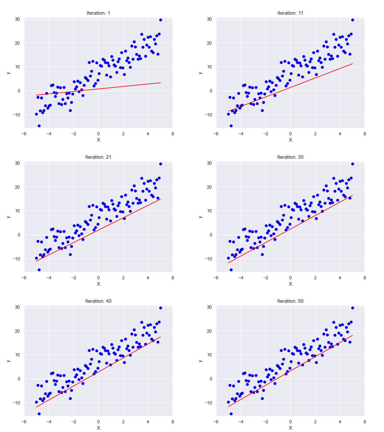
Looking at the graph, you see a general trend – as practice hours increase, so does the batting average. But the relationship is not perfect. The dots do not line up neatly along a straight line but are scattered around. This is where Linear Regression comes in.

Linear Regression finds the ‘line of best fit’ through this scatter of dots. This line represents the average relationship between practice hours and batting averages. So, if a player practices for ‘x’ hours, we can look at the line to predict their batting average. The ‘line of best fit’ is determined mathematically by the method of ‘least squares’, which minimizes the total distance between the line and all the dots.

In the next sections, we’ll get deeper into these concepts. But remember, at its core, Linear Regression is just trying to draw the best straight line through a scatter of dots!

IV. Explaining Key Concepts

In this section, we’re going to talk about some key terms that you need to understand to fully grasp Linear Regression. Think of this as the vocabulary lesson before we start reading the book! Don’t worry, I’ll try to keep it as simple as possible.

1. Independent Variable: This is something that you change or control in your experiment or observation. For example, imagine you are growing plants and you want to see how the amount of sunlight affects their growth. The amount of sunlight would be the independent variable because it’s the factor you are manipulating.
2. Dependent Variable: This is the outcome or results that you measure. In our plant growth example, the height of the plants would be the dependent variable, because it’s the result of the amount of sunlight the plants received.
3. Coefficient: In the context of Linear Regression, a coefficient represents the change in the dependent variable resulting from a one-unit change in the independent variable. In simpler terms, it tells us how much our predicted outcome (like the plant’s height) would change if we changed our independent variable (like the amount of sunlight) by one unit.
4. Residuals: These are the differences between the actual observed values of the dependent variable and the values predicted by our regression model. For our plant example, if our model predicted that a plant would grow 10 inches when it actually grew 12 inches, the residual would be 2 inches.
5. Equation of a line (y = mx + b): In this equation, ‘y’ is the dependent variable (what we’re trying to predict), ‘x’ is the independent variable (what we’re using to make the prediction), ‘m’ is the slope of the line (how much ‘y’ changes for each change in ‘x’), and ‘b’ is the y-intercept (where the line crosses the y-axis). This equation is the heart of Linear Regression!

V. Real-World Example

Let’s put these concepts into practice with a simple, real-world example. Imagine you’re a kid who loves collecting stickers. Over time, you’ve noticed a pattern: the more chores you do at home, the more stickers you seem to get at the end of the week.

Curious (and hoping to boost your sticker collection), you decide to record how many chores you do each week and the number of stickers you receive. You notice that for each chore you do, you get 2 stickers. If you don’t do any chores, you still get 1 sticker because your parents are nice like that!

In this case, the number of chores is the independent variable (‘x’), and the number of stickers is the dependent variable (‘y’). We can use the equation for a line to predict the number of stickers we’ll get based on the number of chores. The equation is y = mx + b, where ‘m’ (the coefficient) is 2 (stickers per chore), and ‘b’ (the y-intercept) is 1 (the sticker you get even if you don’t do any chores).

So, if you did 5 chores, you could predict that you’d get y = 2*5 + 1 = 11 stickers! And if you checked your sticker collection, you’d see that’s exactly right. That’s Linear Regression in action!

In the next section, we’ll introduce a dataset that we’re going to use to demonstrate Linear Regression, just like our sticker-chore example but with more data and using Python!

VI. Introduction to Dataset

In this article, we’ll be using the USA Housing dataset, a real-world dataset that contains information about individual residential properties in various regions across the United States. The dataset includes the following features:

• ‘Avg. Area Income‘: Average income of residents of the city house is located in.
• ‘Avg. Area House Age‘: Average age of houses in the same city.
• ‘Avg. Area Number of Rooms‘: Average number of rooms for houses in the same city.
• ‘Avg. Area Number of Bedrooms‘: Average number of bedrooms for houses in the same city.
• ‘Area Population‘: The population of the city house is located in.
• ‘Price‘: Price of the house.
• ‘Address‘: Address of the houses.

We will use the ‘Avg. Area Income’ feature as our independent variable to predict the ‘Price’ of the houses, which will be our dependent variable.

VII. Applying Linear Regression

First, let’s start by importing the necessary libraries and loading our dataset.

#Import all required packages
import pandas as pd
import numpy as np
from sklearn.model_selection import train_test_split 
from sklearn.linear_model import LinearRegression
from sklearn import metrics

# Load the dataset
dataset = pd.read_csv('USA_Housing.csv')

#Split the data into features and 
X = dataset['Avg. Area Income'].values.reshape(-1,1)
y = dataset['Price'].values.reshape(-1,1)

#Split the data into Test and Train
X_train, X_test, y_train, y_test = train_test_split(X, y, test_size=0.2, random_state=0)

#Train the Model
regressor = LinearRegression()  
regressor.fit(X_train, y_train) #training the algorithm

#To retrieve the intercept:
print(regressor.intercept_)

#For retrieving the slope:
print(regressor.coef_)

#Prediction
y_pred = regressor.predict(X_test)

#Model Evaluation
print('Mean Absolute Error:', metrics.mean_absolute_error(y_test, y_pred))  
print('Mean Squared Error:', metrics.mean_squared_error(y_test, y_pred))  
print('Root Mean Squared Error:', np.sqrt(metrics.mean_squared_error(y_test, y_pred)))

df = pd.DataFrame({'Actual': y_test.flatten(), 'Predicted': y_pred.flatten()})
df = df.round(2)
print(df)

#Visualize the actual vs predicted values (Only First 25 values)
df1 = df.head(25)
df1.plot(kind='bar',figsize=(10,8))
plt.grid(which='major', linestyle='-', linewidth='0.5', color='green')
plt.grid(which='minor', linestyle=':', linewidth='0.5', color='black')
plt.show()

Please explore the code in the Playground section, where you can experiment with it and see the results firsthand.

PLAYGROUND:

VIII. Understanding the Results

Now that we have made predictions using our Linear Regression model, let’s dive into understanding the results and how to interpret them. As mentioned earlier, we have measured the performance of our model using various evaluation metrics. Let’s discuss what these metrics mean and how they help us assess the accuracy of our predictions.

1. Mean Absolute Error (MAE):
   • The MAE measures the average magnitude of errors between the actual and predicted values.
   • In our case, the MAE is 219,728.34. This means that, on average, our model’s predictions are off by approximately $219,728.34.
   • The lower the MAE, the better the model’s performance. However, it’s important to consider the context of the problem and the scale of the target variable.
2. Mean Squared Error (MSE):
   • The MSE calculates the average of the squared differences between the actual and predicted values.
   • Our MSE is 74,084,394,125.46. This value is much larger than the MAE because the errors are squared.
   • Similar to the MAE, a lower MSE indicates better performance, but the scale should be taken into account.
3. Root Mean Squared Error (RMSE):
   • The RMSE is the square root of the MSE and provides a measure of the average magnitude of errors in the same units as the target variable.
   • In our case, the RMSE is 272,184.49. This value represents the average difference between the predicted and actual prices in dollars.
   • Lower RMSE values indicate better accuracy of the model’s predictions.

Interpreting the results:

• In our example, the MAE, MSE, and RMSE values indicate that our model has some degree of prediction error.
• The specific values may vary depending on the dataset and problem domain, but they serve as a reference point for evaluating model performance.
• It’s crucial to compare these metrics with domain-specific knowledge and consider the impact of prediction errors on the problem at hand.

IX. Limitations of Linear Regression

While Linear Regression is a powerful and widely used algorithm, it has certain assumptions and limitations that need to be considered. Understanding these limitations helps us make informed decisions when applying Linear Regression to real-world problems. Here are some key points to keep in mind:

1. Linearity assumption:
   • Linear Regression assumes a linear relationship between the independent variables and the dependent variable.
   • If the true relationship is not linear, the model’s predictions may not be accurate.
   • Techniques such as polynomial regression can be used to capture non-linear relationships.
2. Independence of errors:
   • Linear Regression assumes that the errors (residuals) are independent of each other.
   • If the errors exhibit correlation or patterns, the model may not provide reliable predictions.
   • Techniques like autoregressive models can handle correlated errors.
3. Homoscedasticity:
   • Homoscedasticity implies that the variance of errors is constant across all levels of the independent variables.
   • If the errors show heteroscedasticity, meaning the variance is not constant, the model’s predictions may be biased.
   • Methods such as weighted least squares can address heteroscedasticity.
4. Outliers and influential points:
   • Linear Regression is sensitive to outliers and influential points that can heavily influence the model’s fit.
   • It’s important to identify and handle outliers appropriately to prevent them from skewing the model’s predictions.
5. Multicollinearity:
   • Multicollinearity occurs when independent variables are highly correlated with each other.
   • It can make it difficult to interpret the individual effects of the variables and may affect the stability of the model.
   • Techniques such as regularization or dimensionality reduction can help address multicollinearity.

QUIZ: Test Your Knowledge!