I. INTRODUCTION
Imagine you’re in a park playing a game of hide-and-seek with your friends. Suddenly, you’re ‘it’ and have to find everyone else. With your eyes covered, you have no idea where everyone has hidden. The moment you open your eyes, you see different trees, bushes, and park benches where your friends could be hiding. But where should you start looking?
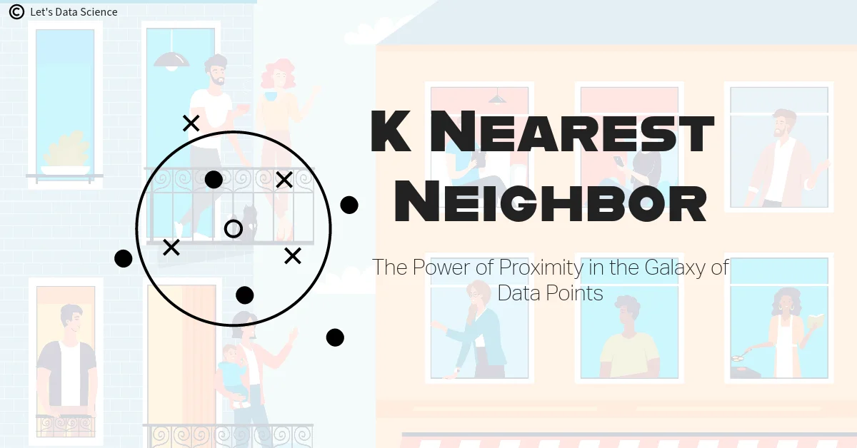
If you’re a smart player, you’ll start by looking at the nearest hiding spots first, right? It makes sense! This idea is the essence of the K-Nearest Neighbors (KNN) algorithm in machine learning. But instead of finding friends in a park, KNN is used to classify new data points based on the data points that are most similar to it, or nearest to it, in a dataset.
Isn’t it exciting that a simple childhood game could help us understand such a powerful machine-learning algorithm? Throughout this article, we’re going to learn more about this KNN ‘game’ – when to use it, why to use it, and how it makes ‘tagging’ or classifying new data points such a breeze!
II. BACKGROUND INFORMATION
Before we jump into our game of KNN hide-and-seek, let’s warm up by recalling some of the other ‘games’ or classification methods we’ve already learned: Logistic Regression and Naive Bayes Classifier.
Just as different games have different rules, each classification method operates differently. In Logistic Regression, we used a formula or equation to predict the probability that a new data point belongs to a certain category or class. On the other hand, the Naive Bayes Classifier is a little more like being a detective, using probabilities and making assumptions about the independence of features to predict the class of a new data point.
Now, what makes KNN different from these two? Well, KNN doesn’t rely on assumptions about data or fit a model using a specific formula. Instead, it uses the concept of ‘distance’ to find the most similar or ‘nearest’ data points in the dataset, much like you would in a game of hide-and-seek!
But just as we need to know the layout of the park to play hide-and-seek effectively, we need to understand some concepts that can affect the performance of KNN, like distance metrics and feature scaling.
Distance metrics help KNN to measure the ‘distance’ or difference between data points. It’s like determining how far one hiding spot is from another in the park. Feature scaling, on the other hand, ensures that all features or data points are on the same scale, or are equally important, similar to making sure that all players follow the same rules in the game.
However, just like every game has its challenges, KNN is not immune to overfitting. Overfitting is like being so good at the game that you can find your friends in seconds, but then struggling when you play in a new park. KNN can also struggle to perform well when it’s too finely tuned to the training data or if the number of neighbors (K) is not chosen correctly.
But don’t worry! We’re going to take a deeper look at these concepts and learn how to handle them effectively. By the end of this article, you’ll be an expert at the KNN game! So, are you ready to begin your journey into the world of K-Nearest Neighbors? Let’s go!
III. HOW KNN CLASSIFIER WORKS
Imagine you’re at a party, and you see a group of people wearing comic book t-shirts and discussing the latest Marvel movie. Nearby, another group is wearing sports jerseys and talking about last night’s football game. If a new person walks into the party wearing a Spider-Man t-shirt, which group do you think they’ll join? You’d probably guess the comic book group, right? This is the basic idea behind the K-Nearest Neighbors (KNN) algorithm.
KNN is like a very observant party-goer. It classifies new data points based on how similar they are to existing data points. Just like you guessed the new person would join the comic book group because they were dressed similarly to that group, KNN guesses the class of new data points based on the ‘K’ number of points that are nearest to it.
In the context of machine learning, the party-goers are data points, the groups are different classes, and the type of clothing is a feature. KNN is a type of ‘lazy learner’ – it doesn’t make any assumptions about the data in advance, and it doesn’t create a model until it’s asked to make a prediction. Then, it simply looks at the ‘K’ number of data points that are closest to the new point, and assigns it to the most common class among those neighbors.
But you might be wondering, how does KNN decide what’s ‘near’ or ‘far’? Well, that’s where distance metrics come in!
IV. UNDERSTANDING DISTANCE METRICS IN KNN
Distance metrics are like the invisible lines we draw when we’re deciding who’s ‘near’ or ‘far’ from us. Just like you might say someone is ‘near’ if they’re in the same room as you, and ‘far’ if they’re in a different city, KNN uses distance metrics to measure how close one data point is to another.
One common distance metric is the ‘Euclidean distance’, named after the ancient Greek mathematician Euclid. Imagine you and your friend are standing in a park, and you want to walk to a tree. The Euclidean distance is like the straight line you’d walk directly from your position to the tree.
Mathematically, if we have two points P1 and P2 in a 2-dimensional space with coordinates (x1, y1) and (x2, y2), the Euclidean distance between them is calculated as √[(x2-x1)² + (y2-y1)²]. In higher dimensions, this formula is extended with more terms, one for each feature.
Another common distance metric is the ‘Manhattan distance’, named after the grid-like layout of Manhattan’s streets. If the tree you want to walk to is at the other end of a football field, you can’t walk straight to it – you have to walk around the field. The Manhattan distance measures this path, going along the grid lines.
In the Manhattan distance, if we have two points P1 and P2 with coordinates (x1, y1) and (x2, y2), the distance between them is calculated as |x2-x1| + |y2-y1|. Like the Euclidean distance, this formula is extended with more terms in higher dimensions.
Choosing the right distance metric is important because it affects how KNN classifies new points. Different distance metrics can give different results, so it’s often a good idea to experiment with a few and see which one works best for your data.
Remember, the goal of KNN and its distance metrics is to take a new data point and find out where it ‘fits in’ – just like figuring out which group a new person at the party might want to join!
V. KEY CONCEPTS IN KNN CLASSIFIER
K-Nearest Neighbors (KNN) Classifier:
Imagine you’re in a city and you see a group of people wearing the same jersey cheering for a soccer match. Even without asking, you can guess they all support the same team, right? This is how KNN works! In KNN, ‘K’ stands for the number of ‘neighbors’ we look at. If most of our ‘neighbors’ belong to a particular group (like wearing the same jersey), we assume that the new person (or data point) also belongs to that group.
Distance Metrics:
Distance metrics are like measuring the distance between two cities. But instead of cities, we measure the distance between data points. If two data points are close together, it means they’re similar. If they’re far apart, they’re different. These distances help KNN decide which group a new data point belongs to.
K parameter:
The ‘K’ in KNN is a number you get to choose. If K is 3, it means we look at the 3 closest neighbors to decide which group a new data point belongs to. The best ‘K’ is not too small and not too big. If you choose K as 1, you’re like a person who only trusts their closest friend’s opinion. If you choose a big K, you’re like a person who asks everyone in the city for their opinion. You want to be somewhere in between!
Overfitting:
Overfitting is like memorizing all the answers for a test. Sure, you might get full marks on that test, but if the questions change slightly, you might fail! In KNN, overfitting happens when we choose a very small K. The model becomes very sensitive to noise and outliers, which may result in poor performance on new, unseen data.
Feature Scaling:
Feature scaling is like converting all your measurements to the same unit before you compare them. You can’t compare 3 pounds to 1000 grams unless you convert them to the same unit. In KNN, we scale all features to the same range so that no feature dominates the others based on its scale.
VI. REAL-WORLD EXAMPLE OF KNN CLASSIFIER
Let’s think about a real-life scenario where KNN can be used. Suppose we’re trying to predict what kind of movies a person will like based on their age and how much they use social media. We have data from lots of people, and we know the types of movies they like.
For instance, we notice that young people who use social media a lot tend to like science fiction movies. On the other hand, older people who don’t use social media much seem to prefer documentaries. Now, let’s say we have a new person who’s young and uses social media a lot. Using KNN, we’d look at other people who are similar in age and social media usage. If most of these people like science fiction movies, we’ll predict that this new person will also like science fiction movies!
Now, in the real world, data scientists use KNN in more complex scenarios. For example, KNN can be used in recommendation systems like suggesting songs on Spotify or products on Amazon. It’s also used in healthcare, for example, to predict the likelihood of a disease based on a patient’s symptoms. Remember, the key to KNN is finding ‘neighbors’ who are similar and using their ‘votes’ to predict the group of a new data point.
VII. INTRODUCTION TO DATASET
For our K-Nearest Neighbors (KNN) Classifier exploration, we’ll be using the well-known “Iris” dataset. The Iris dataset is a classic in the world of data science and machine learning, ideal for classification problems.
The dataset consists of 150 samples from each of three species of Iris flowers (Iris setosa, Iris virginica, and Iris versicolor). Four features were measured from each sample: the lengths and the widths of the sepals and petals. These characteristics make it a fantastic, relatively simple dataset to demonstrate the power of the KNN Classifier.
Each row in the dataset represents an iris flower, including its species and dimensions of its botanical parts, sepal, and petal, in centimeters. If we think of these flowers as ‘neighbors’ in a botanical garden, our job is to classify an unlabelled Iris flower based on these measured features, by looking at its ‘nearest neighbors’, i.e., the flowers which have similar features.
VIII. APPLYING KNN CLASSIFIER
Firstly, we need to import the necessary libraries and load our dataset:
# Importing necessary libraries
from sklearn.datasets import load_iris
from sklearn.model_selection import train_test_split
from sklearn.preprocessing import StandardScaler
from sklearn.neighbors import KNeighborsClassifier
from sklearn.metrics import confusion_matrix, classification_report

# Loading Iris dataset
iris = load_iris()

# Let's print the iris dataset description to understand it better
print(iris.DESCR)

# Splitting dataset into training and testing sets
X_train, X_test, y_train, y_test = train_test_split(iris.data, iris.target, test_size=0.2, random_state=42)

# Let's print the number of instances in each set to verify the split
print(f"Training set has {X_train.shape[0]} instances. Testing set has {X_test.shape[0]} instances.")

#KNN Classifier relies on the distance between feature vectors, so feature scaling is important. Here, we #use StandardScaler to normalize our feature set:
# Creating a StandardScaler instance
sc = StandardScaler()

# Fitting the scaler to the training feature set
X_train = sc.fit_transform(X_train)

# Applying the scaler to the testing feature set
X_test = sc.transform(X_test)

# Creating a KNN instance (let's start with k=5)
knn = KNeighborsClassifier(n_neighbors=5)

# Training the KNN classifier
knn.fit(X_train, y_train)

# Predicting the test set results
y_pred = knn.predict(X_test)

# Creating confusion matrix
cm = confusion_matrix(y_test, y_pred)
print("Confusion Matrix: \n", cm)

# Creating classification report
cr = classification_report(y_test, y_pred)
print("Classification Report: \n", cr)
And voila! You have successfully applied KNN Classifier to the Iris dataset. In the next section, we will interpret these results, and understand the strengths and weaknesses of our KNN Classifier.
PLAYGROUND:
IX. INTERPRETING KNN CLASSIFIER RESULTS
Congratulations on reaching this point! Now, we’re ready to explore the results of our KNN Classifier. We’ll take a look at two important tools that help us understand how well our model performed – the confusion matrix and the classification report. Don’t worry, we’ll break down these big words into simpler terms so that they’re easy to understand.
Let’s start with the confusion matrix. It’s like a report card that tells us how many times our model got the answers right and wrong. For our example, we had three classes to predict (0, 1, and 2). The matrix is a 3×3 table that tells us how our model performed.
Here’s what our matrix is telling us: [[10 0 0] [0 9 0] [0 0 11]]
The rows represent the actual classes, and the columns represent the predicted classes. If we look at the first row (class 0), we can see that all 10 instances were correctly predicted as class 0. There were no instances of wrongly classified. The same goes for the second and third rows (classes 1 and 2). Our model aced the test with a perfect score! This is a sign that our KNN classifier did an exceptional job.
Next up, we have the classification report. This report gives us some crucial metrics, such as precision, recall, and the f1-score. Let’s decode these terms:
- Precision: It tells us about the accuracy of positive predictions. For all three classes (0, 1, and 2), the precision is 1.00, meaning our model made no mistakes when it predicted an instance to belong to these classes.
- Recall: It tells us how many actual positives our model was able to catch. Once again, the recall score for all three classes is 1.00, implying our model perfectly identified all instances of each class.
- F1-score: It is a blend of precision and recall, giving us a single metric that tells us how well our model is doing. An F1 score of 1.00 for all classes indicates an excellent model performance.
In simple terms, our model was a perfect classifier for this dataset – a superstar!
X. COMPARING KNN WITH LOGISTIC REGRESSION AND NAIVE BAYES
Now, it’s time to compare our superstar KNN classifier with the other classification models we’ve learned about Logistic Regression and Naive Bayes. You might be thinking, “Why should we do this if our KNN classifier is already a superstar?” Well, it’s because each of these models has its strengths and weaknesses, and they can perform differently depending on the data.
- Logistic Regression: This model is a bit like the diligent student who likes to study alone. It’s a simple model that works well when there’s a clear linear boundary separating the classes. However, in more complex scenarios, where the classes can’t be separated by a straight line, Logistic Regression might struggle. Also, it doesn’t perform well if there are irrelevant features in the data, as it tries to use all features for the prediction.
- Naive Bayes: This model is like an adventurous kid who loves to explore. It can handle complex datasets with many features quite well. It also works well with text data, making it popular for spam filtering and sentiment analysis. However, it assumes that all features are independent, which is not always the case. For instance, if you’re trying to predict the weather, the temperature and humidity are likely related to each other. Naive Bayes might struggle with such dependent features.
- KNN Classifier: Our superstar model is a very social learner. It likes to take votes from its neighbors to make predictions. It works well with smaller datasets and when the classes are tightly clustered together. However, it can be slow and require more computational resources when working with large datasets.
In conclusion, choosing the right model depends on your data and the specific problem you’re trying to solve. Sometimes, you might need the diligent nature of Logistic Regression, other times the adventurous spirit of Naive Bayes, and occasionally, the social nature of the KNN Classifier might be just what you need.
XI. LIMITATIONS AND ADVANTAGES OF KNN CLASSIFIER
Let’s imagine KNN as a superhero named “Kaptain KNN”. Now, like all superheroes, Kaptain KNN has some special powers (advantages) and some weaknesses (limitations). Understanding these will help us know when to call upon Kaptain KNN and when we might want to choose a different superhero to save the day.
ADVANTAGES OF KNN CLASSIFIER:
- Simple and Intuitive: Think of Kaptain KNN as the friendly neighborhood hero. His powers are easy to understand. He makes decisions based on the majority vote of his nearest neighbors. No fancy tricks, no complex calculations.
- No Assumptions Needed: Some superheroes need the right conditions to work best. For example, many machine learning models assume that data is normally distributed or that features are independent. But not Kaptain KNN! He is flexible and works with any kind of data.
- Learning on the Go: Kaptain KNN is always learning. He doesn’t create a model of the world and stick to it. Instead, he makes decisions on the fly based on the most up-to-date data. This is known as “lazy learning”.
LIMITATIONS OF KNN CLASSIFIER:
- Slow in Big Cities (Large Datasets): Kaptain KNN can take a lot of time to make a decision when there’s a lot of data. He insists on considering all of his neighbors before making a decision, and this can take a long time when there are many neighbors.
- Gets Confused by Irrelevant Neighbors (Noisy Data): Sometimes, Kaptain KNN can get confused if his neighbors give him misleading information. If the data is noisy or if there are irrelevant features, Kaptain KNN might make the wrong decision.
- Sensitive to Unfair Comparisons (Feature Scaling): Kaptain KNN likes to compare things fairly. If one type of data (like weight) is in a much larger scale than another type (like height), he might give too much importance to the larger one. So, it’s important to normalize or scale the data before calling Kaptain KNN into action.
In short, Kaptain KNN is a great superhero to have on our team, but we should be aware of his strengths and weaknesses to make the best use of his powers.
XII. CONCLUSION
As we come to the end of our journey, we now have a new friend in Kaptain KNN! We’ve seen how he makes decisions based on the wisdom of his neighbors. We’ve learned about his special powers and his limitations.
Remember, no one superhero is the best in all situations. Kaptain KNN is perfect for some tasks, but not all. It’s important to know when to call upon him and when to seek help from other superheroes like Logistic Regression or Naive Bayes.
Stay tuned for our next adventure where we’ll meet more superheroes in the world of machine learning. Next up, we’re entering the forest to meet an entire team of heroes – the Decision Trees and their powerful ensemble, the Random Forest!
So, fasten your seat belts, and get ready for the next exciting journey into the world of machine learning!
QUIZ: Test Your Knowledge!
0 of 20 Questions completed Questions: You have already completed the quiz before. Hence you can not start it again.
Quiz is loading… You must sign in or sign up to start the quiz. You must first complete the following:
0 of 20 Questions answered correctly
Your time:
Time has elapsed
You have reached 0 of 0 point(s), (0)
Earned Point(s): 0 of 0, (0) What is the essence of the K-Nearest Neighbors (KNN) algorithm in machine learning? Which classification method does not rely on assumptions about data or fit a model using a specific formula? What concept in KNN helps measure the ‘distance’ or difference between data points? Which distance metric in KNN is named after the ancient Greek mathematician Euclid? What does the ‘K’ in K-Nearest Neighbors (KNN) represent? What is overfitting in the context of KNN? Why is feature scaling important in K-Nearest Neighbors (KNN)? What is a real-world example where KNN can be used? Which dataset is used in the example to demonstrate the K-Nearest Neighbors (KNN) Classifier? What does the confusion matrix in KNN tell us? Which metric in the classification report tells us about the accuracy of positive predictions? What is a limitation of K-Nearest Neighbors (KNN) Classifier? Which classification model is like the diligent student who works well when there’s a clear linear boundary separating the classes? What superhero is used as an analogy to describe the K-Nearest Neighbors (KNN) Classifier? Why is K-Nearest Neighbors (KNN) considered a ‘lazy learner’? What is the key advantage of K-Nearest Neighbors (KNN) Classifier? Which distance metric in KNN is named after the grid-like layout of Manhattan’s streets? What does the ‘K’ parameter in K-Nearest Neighbors (KNN) represent? Which metric in the classification report tells us how well our model is performing? What is a limitation of K-Nearest Neighbors (KNN) Classifier when working with large datasets?
Quiz Summary
Information
Results
Results
0 Essay(s) Pending (Possible Point(s): 0)
Categories
1. Question
2. Question
3. Question
4. Question
5. Question
6. Question
7. Question
8. Question
9. Question
10. Question
11. Question
12. Question
13. Question
14. Question
15. Question
16. Question
17. Question
18. Question
19. Question
20. Question


